For physical computing or amateur science projects, you often need to be able to get the output of a sensor or transducer into your computer. There are a lot of ways to do this with specialized data acquisition hardware and software. This method is pretty old school, and requires only a standard laptop and a handful of inexpensive electronic components. It may be appropriate if you are working in a relatively quiet environment and you don’t need to take a lot of samples per second.
Just about any physical signal or measurement in the world can be converted into a fluctuating voltage, an analog signal. Most laptops have a built-in microphone, so if you can convert your voltage into an audible signal, you can use the microphone to digitize it. Once it is in digital form, you can then process the signal with any programming language. Here we’ll use Mathematica.
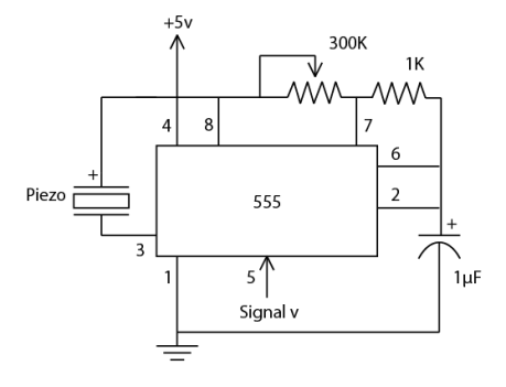
The electronic side of the project is a very simple metronome (or tone generator) based on the 555 timer. It is a mashup of two circuits from Forrest Mims’ work, the V/F Converter on page 51 of his Science and Communication Circuits and Projects and the Audio Oscillator / Metronome on p. 22 of his Timer, Op Amp and Optoelectronic Circuits and Projects.
The changing voltage from a sensor or transducer is fed into pin 5 on the timer. For voltages between about 1.25v and 4.70v, the timer will respond with chirps or clicks that are more-or-less frequent: the frequency depends on the voltage. With lower voltages, the frequency is higher, and with higher voltages it is lower. The variable resistor can be used to tune the center of the frequency range. Increasing the value of the capacitor decreases the frequency and makes each individual chirp longer. Decreasing the value of the capacitor increases the frequency and makes each chirp shorter. For the test here, the variable resistor was set to 100K measured with a digital multimeter. The piezo element was rated for 3-20v, 10mA. You can make the circuit portable by powering it with a 9v battery, but you might have to adjust the values of the resistors and capacitor for best results. I used a bench power supply and proto-board for my experiments.
To make a sample signal, I connected the signal line to a power supply set at 4.7v, decreased it by hand to 1.25v, then increased it back to 4.7v. The circuit responded by producing slower, faster and slower clicks. If you would like to listen to the recording, there are MP3 and WAV files in the GitHub repository.
My original plan was to use the SystemDialogInput[ “RecordSound” ] command to record the audio directly into Mathematica, but that feature is unfortunately not supported on Macs yet. So I recorded the sample using Audacity instead, and then used the Import command to load the sound file into Mathematica.
My complete Mathematica notebook is available for download on GitHub. Here are the highlights.
We load the signal in as data, and plot every thousandth point to get an idea of what it looks like. Since we sampled the sound at 44100 Hz, there will be 44100 data points for each second of audio, or 44.1 data points per millisecond. The duration of each click is on the order of 10 milliseconds or less, so we won’t be able to make out individual clicks this way.
signalData = Flatten@Import[path <> "sample-data.wav", "Data"];
ListLinePlot[
   signalData[[1 ;; Length[signalData] ;; 1000]],
   ImageSize -> Full, AspectRatio -> 0.25, PlotRange -> All,
   Joined -> False, Filling -> Axis]
 Near the beginning of the sample, the clicks are relatively sparse. If we start at the 3 second mark and plot every point for 50 milliseconds of our data, we can see one click.
second=44100;
msec=N[second/1000];
sparseRegion=signalData[[(3*second) ;; (3*second) + Round[50*msec]]];
ListLinePlot[sparseRegion,
    ImageSize -> Full, AspectRatio -> 0.25, PlotRange -> All,
    Joined -> False, Filling -> Axis]
 We are interested in pulling out the clicks, so we take the absolute value of our data, then use the MovingAverage command to smooth it a bit. Averaging over ten data points seems to give us a sharp peak.
ListLinePlot[MovingAverage[Abs[sparseRegion], 10],
    ImageSize -> Full, AspectRatio -> 0.25, PlotRange -> All,
    Joined -> False, Filling -> Axis]
Now we can use a thresholding function that returns 1 when the signal is above a given level and 0 otherwise. We use Map to apply the function to each data point.
thresholdFunction[value_, threshold_] :=
    If[value > threshold, 1, 0]
threshold = 0.25;
ListLinePlot[
    Map[
        thresholdFunction[#, threshold] &,
        MovingAverage[Abs[sparseRegion], 10]],
    ImageSize -> Full, AspectRatio -> 0.25, PlotRange -> All,
    Joined -> False, Filling -> Axis]
This looks pretty good when the clicks are infrequent. We need to make sure that it will work in a region of our signal where clicks are more frequent, too. We look at a 50-millisecond-long region 10 seconds into our signal, doing the same processing and plotting the results.
denseRegion=signalData[[(10*second) ;; (10*second) + Round[50*msec]]];
Since our thresholding looks like it will work nicely for our data, we can apply it to the whole dataset.
signalThresholded =
    Map[thresholdFunction[#, threshold] &,
        MovingAverage[Abs[signalData], 10]];
Now we need to count the number of clicks that occur in a given interval of time. We will do this by using the Partition command to partition our data into short, overlapping windows. Each window will be 200 milliseconds long, and will overlap those on its left and right by 100 milliseconds each. To count clicks, we will use the Split command to split each window into runs of similar characters (i.e., all 1s or all 0s) then Map the Total function over each of the resulting lists. If there are more than, say, five 1s in a row, surrounded on either side by a run of 0s, we can assume that a click has occurred.
signalThresholdedPartition =
    Partition[signalThresholded, Round[200*msec], Round[100*msec]];
countClicks[window_] :=
    Total[
        Map[If[# > 5, 1, 0] &,
            Map[Total, Split[window]]]]
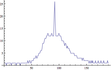
We can now plot the number of clicks per window. This shows us that the voltage starts high, drops, then increases again. Note the spike in the middle, which represents a dense cluster of clicks. Looking at the raw signal, this appears to have been a burst of noise. At this point, we have a workable way to convert a varying voltage into a digital signal that we can analyze with Mathematica. For most applications, the next step would be to calibrate the system by recording audio samples for specific voltages and determining how many clicks per window was associated with each.
ListLinePlot[Map[countClicks, signalThresholdedPartition]]


You must be logged in to post a comment.