(If you have Mathematica you can download this as a notebook from my GitHub account. It is also available as a CDF document which can be read with Wolfram’s free CDF Player.)
Introduction
For a couple of years now I have been using Mathematica as my programming language of choice for my digital history work. For one thing, I love working with notebooks, which allow me to mix prose, citations, live data, executable code, manipulable simulations and other elements in a single document. I also love the generality of Mathematica. For any kind of technical work, there is usually a well-developed body of theory that is expressed in objects drawn from some branch of mathematics. Chances are, Mathematica already has a large number of high-level functions for working with those mathematical objects. The Mathematica documentation is excellent, if necessarily sprawling, since there are literally thousands of commands. The challenge is usually to find the commands that you need to solve a given problem. Since few Mathematica programmers seem to be working historians or humanists dealing with textual sources, it can be difficult to figure out where to begin.
Using a built-in text
As a sample text, we will use the Darwin’s Origin of Species from Mathematica‘s built-in example database. The Short command shows a small piece of something large. Here we’re asking to see the two lines at the beginning and end of this text.
sample = ExampleData[{"Text", "OriginOfSpecies"}];
Short[sample, 2]
Mathematica responds with
INTRODUCTION. When on board H.M.S. ... have been, and are being, evolved.
The Head command tells us what something is. Our text is currently a string, an ordered sequence of characters.
Head[sample]
String
Extracting part of a string
Suppose we want to work with part of the text. We can extract the Introduction of Origin by pulling out everything between “INTRODUCTION” and “CHAPTER 1”. The command that we use to extract part of a string is called StringCases. Once we have extracted the Introduction, we want to check to make sure that the command worked the way we expected. Rather than look at the whole text right now, we can use the Short command to show us about five line of the text. It returns a couple of phrases at the beginning and end, using ellipses to indicate the much larger portion which we are not seeing.
intro=StringCases[sample,Shortest["INTRODUCTION"~~__~~"CHAPTER"]][[1]];
Short[intro,5]
INTRODUCTION. When on board H.M.S. 'Beagle,' as naturalist, I was much struck with certain fac... nced that Natural Selection has been the main but not exclusive means of modification. CHAPTER
Note the use of the Shortest command in the string matching expression above. Since there are probably multiple copies of the word “CHAPTER” in the text, we have to tell Mathematica how much of the text we want to match… do we want the portion between “INTRODUCTION” and the first instance of the word, the second, the last? Here are two examples to consider:
StringCases["bananarama","b"~~__~~"a"]
{bananarama}
StringCases["bananarama",Shortest["b"~~__~~"a"]]
{bana}
From a string to a list of words
It will be easier for us to analyze the text if we turn it into a list of words. In order to eliminate punctuation, I am going to get rid of everything that is not a word character. Note that doing things this way turns the abbreviation “H.M.S.” into three separate words.
introList=StringSplit[intro,Except[WordCharacter]..];
Short[introList,4]
{INTRODUCTION,When,on,board,H,M,S,Beagle,as,<>,the,main,but,not,exclusive,means,of,modification,CHAPTER}
Mathematica has a number of commands for selecting elements from lists. The Take command allows us to extract a given number of items from the beginning of a list.
Take[introList,40]
{INTRODUCTION,When,on,board,H,M,S,Beagle,as,naturalist,I,was,much,struck,
with,certain,facts,in,the,distribution,of,the,inhabitants,of,South,America,
and,in,the,geological,relations,of,the,present,to,the,past,inhabitants,
of,that}
The First command returns the first item in a list, and the Rest command returns everything but the first element. The Last command returns the last item.
First[introList]
INTRODUCTION
Short[Rest[introList]]
{When,on,<>,modification,CHAPTER}
Last[introList]
CHAPTER
We can also use an index to pull out list elements.
introList[[8]]
Beagle
We can test whether or not a given item is a member of a list with the MemberQ command.
MemberQ[introList, "naturalist"]
True
MemberQ[introList, "naturist"]
False
Processing each element in a list
If we want to apply some kind of function to every element in a list, the most natural way to accomplish this in Mathematica is with the Map command. Here we show three examples using the first 40 words of the Introduction. Note that Map returns a new list rather than altering the original one.
Map[ToUpperCase, Take[introList, 40]]
{INTRODUCTION,WHEN,ON,BOARD,H,M,S,BEAGLE,AS,NATURALIST,I,WAS,MUCH,STRUCK,
WITH,CERTAIN,FACTS,IN,THE,DISTRIBUTION,OF,THE,INHABITANTS,OF,SOUTH,AMERICA,
AND,IN,THE,GEOLOGICAL,RELATIONS,OF,THE,PRESENT,TO,THE,PAST,INHABITANTS,OF,
THAT}
Map[ToLowerCase, Take[introList, 40]]
{introduction,when,on,board,h,m,s,beagle,as,naturalist,i,was,much,struck,
with,certain,facts,in,the,distribution,of,the,inhabitants,of,south,america,
and,in,the,geological,relations,of,the,present,to,the,past,inhabitants,of,
that}
Map[StringLength, Take[introList, 40]]
{12,4,2,5,1,1,1,6,2,10,1,3,4,6,4,7,5,2,3,12,2,3,11,2,5,7,3,2,3,10,9,2,3,7,
2,3,4,11,2,4}
Computing word frequencies
In order to compute word frequencies, we first convert all words to lowercase, the sort them and count how often each appears using the Tally command. This gives us a list of lists, where each of the smaller lists contains a single word and its frequency.
lowerIntroList=Map[ToLowerCase,introList];
sortedIntroList=Sort[lowerIntroList];
wordFreq=Tally[sortedIntroList];
Short[wordFreq]
{{1837,1},{1844,2},<>,{years,3},{yet,2}}
Finally we can sort our tally list by the frequency of each item. This is traditionally done in descending order. In Mathematica we can change the sort order by passing the Sort command an anonymous function. (It isn’t crucial for this example to understand exactly how this works, but it is explained in the next section if you are curious. If not, just skip ahead.)
sortedFrequencyList = Sort[wordFreq, #1[[2]] > #2[[2]] &];
Short[sortedFrequencyList, 8]
{{the,100},{of,91},{to,54},{and,52},{i,44},{in,37},{that,27},{a,24},
{this,20},{it,20},{be,20},{which,18},<>,{admiration,1},{admirably,1},
{adduced,1},{adapted,1},{acquire,1},{acknowledging,1},{acknowledged,1},
{accuracy,1},{account,1},{absolutely,1},{1837,1}}
Here are the twenty most frequent words:
Take[sortedFrequencyList, 20]
{{"the", 100}, {"of", 91}, {"to", 54}, {"and", 52}, {"i", 44},
{"in", 37}, {"that", 27}, {"a", 24}, {"this", 20}, {"it", 20},
{"be", 20}, {"which", 18}, {"have", 18}, {"species", 17},
{"on", 17}, {"is", 17}, {"as", 17}, {"my", 13}, {"been", 13},
{"for", 11}}
The Cases statement pulls every item from a list that matches a pattern. Here we are looking to see how often the word “modification” appears.
Cases[wordFreq, {"modification", _}]
{{"modification", 4}}
Aside: Anonymous Functions
Most programming languages let you define new functions, and Mathematica is no exception. You can use these new functions with built-in commands like Map.
plus2[x_]:=
Return[x+2]

Map[plus2, {1, 2, 3}]
{3, 4, 5}
Being able to define functions allows you to
- hide details: as long as you can use a function like plus2 you may not care how it works
- reuse and share code: so you don’t have to keep reinventing the wheel.
In Mathematica, you can also create anonymous functions. One way of writing an anonymous function in Mathematica is to use a Slot in place of a variable.
# + 2 &
So we don’t have to define our function in advance, we can just write it where we need it.
Map[# + 2 &, {1, 2, 3}]
{3, 4, 5}
We can apply an anonymous function to an argument like this, and Mathematica will return the number 42.
(# + 2 &)[40]
A named function like plus2 is still sitting there when we’re done with it. An anonymous function disappears immediately after use.
N-grams
The Partition command can be used to create n-grams. This tells Mathematica to give us all of the partitions of a list that are two elements long and that are offset by one.
bigrams = Partition[lowerIntroList, 2, 1];
Short[bigrams, 8]
{{introduction,when},{when,on},{on,board},{board,h},{h,m},{m,s},{s,beagle},
{beagle,as},{as,naturalist},<>,{been,the},{the,main},{main,but},
{but,not},{not,exclusive},{exclusive,means},{means,of},{of,modification},
{modification,chapter}}
We can tally and sort bigrams, too.
sortedBigrams = Sort[Tally[bigrams], #1[[2]] > #2[[2]] &];
Short[sortedBigrams, 8]
{{{of,the},21},{{in,the},13},{{i,have},11},{{to,the},11},{{which,i},7},
{{to,me},7},{{of,species},6},{{i,shall},5},<>,{{beagle,as},1},
{{s,beagle},1},{{m,s},1},{{h,m},1},{{board,h},1},{{on,board},1},
{{when,on},1},{{introduction,when},1}}
Concordance (Keyword in Context)
A concordance shows keywords in the context of surrounding words. We can make one of these quite easily if we starting by generating n-grams. Then we use Cases to pull out all of the 5-grams in the Introduction that have “organic” as the middle word (for example), and format the output with the TableForm command.
fivegrams=Partition[lowerIntroList,5,1];
TableForm[Cases[fivegrams,{_,_,"organic",_,_}]]
affinities of    organic beings on
several distinct organic beings by
coadaptations of organic beings to
amongst all      organic beings throughout
succession of    organic beings throughout
Removing stop words
Mathematica has access to a lot of built-in, curated data. Here we grab a list of English stopwords.
stopWords = WordData[All, "Stopwords"];
Short[stopWords, 4]
{0,1,2,3,4,5,6,7,8,9,a,A,about,above,<<234>>,with,within,without,would,x,X,y,Y,yet,you,your,yours,z,Z}
The Select command allows us to use a function to pull items from a list. We want everything that is not a member of the list of stop words.
Short[lowerIntroList, 8]
{introduction,when,on,board,h,m,s,beagle,as,naturalist,i,was,much,struck,
with,certain,facts,in,the,<<1676>>,species,furthermore,i,am,convinced,
that,natural,selection,has,been,the,main,but,not,exclusive,means,of,
modification,chapter}
lowerIntroNoStopwords =
  Select[lowerIntroList, Not[MemberQ[stopWords, #]] &];
Short[lowerIntroNoStopwords, 8]
{introduction,board,beagle,naturalist,struck,certain,facts,distribution,
inhabitants,south,america,geological,relations,present<<697>>,species,
descendants,species,furthermore,am,convinced,natural,selection,main,
exclusive,means,modification,chapter}
Bigrams containing the most frequent words
Here is a more complicated example built mostly from functions we’ve already seen. We start by finding the ten most frequently occuring words once we have gotten rid of stop words.
freqWordCounts =
 Take[Sort[
   Tally[Take[
     lowerIntroNoStopwords, {1, -120}]], #1[[2]] > #2[[2]] &], 10]
{{shall,9},{species,9},{facts,9},{chapter,5},{variation,5},
{conditions,5},{beings,5},{organic,5},{conclusions,5},{subject,5}}
We remove a few of the words we are not interested in, then we rewrite the bigrams as a list of graph edges. This will be useful for visualizing the results as a network.
freqWords =
  Complement[Map[First, freqWordCounts], {"shall", "subject"}];
edgeList =
  Map[#[[1]] -> #[[2]] &, Partition[lowerIntroNoStopwords, 2, 1]];
Short[edgeList, 4]
{introduction->board,board->beagle,beagle->naturalist,<<717>>,
exclusive->means,means->modification,modification->chapter}
We grab the most frequent ones.
freqBigrams = Union[Select[edgeList, MemberQ[freqWords, #[[1]]] &],
   Select[edgeList, MemberQ[freqWords, #[[2]]] &]];
Short[freqBigrams, 4]
{abstract->variation,affinities->organic,allied->species,<<87>>,varieties->species,varying->conditions,volume->facts}
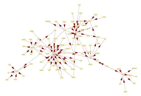
Finally we can visualize the results as a network. When you are exploring a text this way, you often want to keep tweaking your parameters and see if anything interesting comes up.
Framed[Pane[
  GraphPlot[freqBigrams,
   Method -> {"SpringElectricalEmbedding",
     "InferentialDistance" -> .1, "RepulsiveForcePower" -> -4},
   VertexLabeling -> True, DirectedEdges -> True,
   ImageSize -> {1100, 800}], {400, 400}, Scrollbars -> True,
  ScrollPosition -> {400, 200}]]
Document frequencies
We have been looking at the Introduction to Origin. We can also calculate word frequencies for the whole document. When we list the fifty most common words (not including stop words) we can get a better sense of what the whole book is about.
sampleList =
  Map[ToLowerCase, StringSplit[sample, Except[WordCharacter] ..]];
docFreq = Sort[Tally[Sort[sampleList]], #1[[2]] > #2[[2]] &];
Take[Select[Take[docFreq, 200],
  Not[MemberQ[stopWords, First[#]]] &], 50]
{{species,1489},{forms,397},{varieties,396},{selection,383},
{natural,361},{life,298},{plants,297},{different,282},{case,281},
{animals,280},{great,260},{distinct,255},{nature,253},{having,252},
{new,244},{long,243},{period,238},{cases,224},{believe,216},
{structure,214},{conditions,211},{genera,210},{generally,199},
{number,198},{common,194},{far,193},{time,191},{degree,190},
{groups,173},{characters,170},{certain,169},{view,168},{large,168},
{instance,165},{modification,161},{facts,157},{closely,155},
{parts,154},{intermediate,154},{modified,153},{genus,147},
{present,143},{birds,143},{produced,141},{individuals,140},
{inhabitants,139},{parent,138},{world,136},{character,136},
{organic,135}}
TF-IDF: Term frequency-Inverse document frequency
The basic intuition behind tf-idf is as follows…
- A word that occurs frequently on every page doesn’t tell you anything special about that page. It is a stop word.
- A word that occurs only a few times in the whole document or corpus can be ignored.
- A word that occurs a number of times on one page but is relatively rare in the document or corpus overall can give you some idea what the page is about.
Here is one way to calculate tf-idf (there are lots of different versions)
tfidf[termfreq_,docfreq_,numdocs_]:=
     Log[termfreq+1.0] Log[numdocs/docfreq]
Using document frequencies and TF-IDF we can get a sense of what different parts of a text are about. Here is how we would analyze chapter 9 (there are 15 chapters in all).
ch9 = StringCases[sample, Shortest["CHAPTER 9" ~~ __ ~~ "CHAPTER"]][[
   1]];
ch9List = Map[ToLowerCase, StringSplit[ch9, Except[WordCharacter] ..]];
ch9Terms = Union[ch9List];
ch9TermFreq = Sort[Tally[ch9List], #1[[2]] > #2[[2]] &];
ch9DocFreq = Select[docFreq, MemberQ[ch9Terms, #[[1]]] &];
computeTFIDF[termlist_, tflist_, dflist_] :=
 Module[{outlist, tf, df},
  outlist = {};
  Do[
   tf = Cases[tflist, {t, x_} -> x][[1]];
   df = Cases[dflist, {t, x_} -> x][[1]];
   outlist = Append[outlist, {t, tf, df, tfidf[tf, df, 15.0]}],
   {t, termlist}];
  Return[outlist]]
ch9TFIDF =
  Sort[computeTFIDF[ch9Terms, ch9TermFreq,
    ch9DocFreq], #1[[4]] > #2[[4]] &];
Take[ch9TFIDF, 50][[All, 1]]
{teleostean,tapir,richest,pebbles,mississippi,downs,decay,conchologists,
wear,thinner,tear,supplement,superimposed,sedgwick,rolled,poorness,nodules,
mineralogical,levels,inadequate,grinding,gravel,downward,denuded,comprehend,
chthamalus,atom,accumulations,sand,ramsay,littoral,sedimentary,wears,wearing,
wealden,watermark,watch,vehemently,valve,upright,unimproved,unfathomable,
undermined,underlies,unanimously,ubiquitous,transmutation,tides,tidal,swarmed}
Whether or not you are familiar with nineteenth-century science, it should be clear that the chapter has something to do with geology. Darwin also provided chapter summaries of his own:
StringTake[ch9, 548]
CHAPTER 9. ON THE IMPERFECTION OF THE GEOLOGICAL RECORD. On the absence
of intermediate varieties at the present day. On the nature of extinct
intermediate varieties; on their number. On the vast lapse of time, as
inferred from the rate of deposition and of denudation. On the poorness
of our palaeontological collections. On the intermittence of geological
formations. On the absence of intermediate varieties in any one formation.
On the sudden appearance of groups of species. On their sudden appearance
in the lowest known fossiliferous strata.


You must be logged in to post a comment.