Introduction

In the previous post, we used command line tools to manipulate and study text files that contained rows and columns of data, some numeric. These kind of files are often known as CSV files–for “comma separated values”–even though the separators may be other punctuation characters, tabs or spaces. Putting data into CSV format is one way of structuring it, while still allowing it to be stored in a human- and machine-readable file. Not all data lends itself to being laid out in rows and columns, however. A different strategy for representing structure is to provide markup in the form of tags that indicate how a region of text should be displayed, what it means, or some other associated metadata. If these metadata tags are stored in the same file as the text to which they refer, they need to be syntactically distinguished from their surroundings. That is to say, it should be perfectly clear to a human or machine reader which part of the file is text and which part is tag. Here are some examples. The sentence below has two HTML (HyperText Markup Language) tags which indicate how it should be displayed in a web browser. Note the use of angle brackets and a forward slash to indicate which is the beginning tag and which is the ending one.

This is how you indicate <em>emphasis</em>, and this is how you make something <strong>stand out</strong> from its surroundings.

In XML (Extensible Markup Language), you can create tags to represent any kind of metadata you wish.

The field notes were written by <author>Frank N. Meyer</author>.

In HTML and XML, tags should be properly nested.

<outside_tag>This is <inside_tag>properly nested</inside_tag></outside_tag>
<outside_tag>This is <inside_tag>not properly nested</outside_tag></inside_tag>

[UPDATE 2014. This post was changed slightly to reflect changes in WorldCat records that were made since the original post. The sense of the lesson is unchanged.]

Installation

Since markup files are plain text, we can use Linux command line tools like cat, tr, sed, awk and vi to work with them. It turns out to be sometimes difficult to match tags with regular expressions, however, so working with grep can be frustrating. We will install a special utility called xmlstarlet to alleviate some of these problems. Use man to see if you have xmlstarlet installed. If not, install it with

sudo aptitude install xmlstarlet

[UPDATE 2014. If you are using HistoryCrawler you will have to install xmlstarlet but not graphviz.]

Later in this post we are also going to visualize some relationships in the form of graphs, diagrams that show lines or arrows connecting points or labeled nodes. We will use the graphviz package for this. Use man to see if you have it installed. If not, install it with

sudo aptitude install graphviz

Getting an XML document and extracting elements

In previous posts (1, 2), we spent some time looking at the field notes written by Frank N. Meyer during a USDA-sponsored botanical expedition to South China, 1916-18. Here we are going to use the OCLC WorldCat Identities database to learn more about Meyer and the people with whom he was associated. OCLC, the Online Computer Library Center, is the organization  that maintains WorldCat, a union catalog of the holdings of tens of thousands of libraries worldwide. The Identities database contains records of the 30 million persons, organizations, fictitious characters, and so on that the items in WorldCat are by or about. Start your GUI, open a terminal and start the iceweasel (or Firefox) browser in the background. The Identities page for Frank N. Meyer is at http://www.worldcat.org/identities/lccn-n83-126466. Spend some time exploring the page so you know what is on it. Now, in a new browser tab, open the XML version of the same page at http://www.worldcat.org/identities/lccn-n83-126466/identity.xml. Spend some time comparing the two pages. You want to discover how information that is presented for human consumption in the regular webpage is encoded in human- and machine-readable tags in the XML page. Note that you should be able to expand and collapse XML tags in your web browser display. In iceweasel, you do this by clicking on the little minus signs beside a particular tag. Doing this will give you a better sense of how the tags are nested. Now that we have a sense of the structure of the XML document, we can try extracting some of this information using command line tools. In the terminal, use wget to download a local copy of the XML file, then use the xmlstarlet el command to get a listing of the elements in the file.

wget http://www.worldcat.org/identities/lccn-n83-126466/identity.xml
xmlstarlet el identity.xml | less

Note that for associated names, we see the following pattern repeated:

Identity/associatedNames/name
Identity/associatedNames/name/normName
Identity/associatedNames/name/rawName
Identity/associatedNames/name/rawName/suba
Identity/associatedNames/name/rawName/subb
Identity/associatedNames/name/rawName/subd

Each of these lines represents a ‘path’ to a particular element in the XML document. Looking at the XML display in iceweasel we can see how associated names are tagged. We see that the normName field contains the LCCN. This is the Library of Congress Control Number, a unique identifier. Frank N. Meyer’s LCCN is n83126466. The human-readable name is stored in the rawName/suba field, with optional information in rawName/subb. Dates are in rawName/subd.

Selecting information from an XML document

We can pull information out of an XML file using the xmlstarlet sel command. For example, if we wanted to count the number of associated names, we would type the following. The -t option tells xmlstarlet to return plain text; the -v (value) option tells it what we are looking for.

xmlstarlet sel -t -v "count(/Identity/associatedNames/name)" -n identity.xml

Here we are more interested in using xmlstarlet to parse the XML file, that is, to find information and extract it. As a first attempt, we try matching (-m) the associated names and pulling out the values (-v) of the normName fields. The -n option puts newlines where we want them.

xmlstarlet sel -t -m "/Identity/associatedNames/name" -v "normName" -n identity.xml

The output that we get looks like the following.

lccn-n79008243
lccn-n83126465
lccn-n80145310
nc-united states$government printing office
lccn-n85140459
lccn-n85335475
lccn-n50015525
np-kelsey, harlan p
lccn-n79076676
lccn-n85800990

While we are at it, we can also grab information from the rawName fields. We modify our command to do that, outputting the results in a colon-separated table. The -T option says we want to output plain text. The -o option provides our output separators. Note that we are also including escaped quotation marks around our name fields. This will help us later when we further manipulate the information we are extracting.

xmlstarlet sel -T -t -m "/Identity/associatedNames/name" -v "normName"  -o ":\"" -v "rawName/suba" -o " " -v "rawName/subb" -o "\"" -n identity.xml

Our output now looks like this:

lccn-n79008243:"United States Dept. of Agriculture"
lccn-n83126465:"Cunningham, Isabel Shipley "
lccn-n80145310:"United States Bureau of Plant Industry"
...
lccn-n85800990:"Smith, Erwin F. "

The blank spaces in the rawName fields will cause us problems later, so we are going to use tr to eliminate those. We will use grep to get rid of the entries that don’t have proper LCCNs. Finally, we will package everything up into a convenient Bash shell script. Use a text editor to create the following file, and name it get-assoc-names.sh.

#! /bin/bash

xmlstarlet sel -T -t -m "/Identity/associatedNames/name" -v "normName"  -o ":\"" -v "rawName/suba" -o " " -v "rawName/subb" -o "\"" -n $1 | grep 'lccn' | tr -d ' '

Now you can change the permissions and try executing the script as follows. The last command shows how you can use cut to pull out just the names.

chmod 744 get-assoc-names.sh
./get-assoc-names.sh identity.xml
./get-assoc-names.sh identity.xml | cut -d':' -f2

We can also write a small script to pull out the LCCN and rawName for the identity that the file is about (in this case, Frank N. Meyer). Look at the XML display in your browser again. In this case, we have to use the ‘@’ character to specify the value for a tag attribute. Use a text editor to write the following script, save it as get-name.sh, change the file permissions and try executing it.

#! /bin/bash

xmlstarlet sel -T -t -v "/Identity/pnkey" -o ":\"" -v "/Identity/nameInfo[@type='personal']/rawName/suba" -o "\"" -n $1 | tr -d ' '

Plotting a directed graph

If we want to visualize the relationships between a set of entities, one way is to create a graphical figure that shows the entities as dots or nodes, and the relationships as lines or arrows. In mathematics, this kind of figure is known as a graph (not to be confused with the other sense of the word, which usually refers to the plot of a function’s output). If the connection between two entities is directional (an arrow, rather than a line), the graph is called a digraph, or directed graph. Suppose that John Doe has some kind of relationship to Jane Doe: he might be her son, nephew, husband, uncle, Facebook friend, whatever. If we want to visualize this relationship with the Graphviz software package, we start by creating a file that looks like the following. Use a text editor to create the file and save it as example.dot.

digraph G {
     "JohnDoe" -> "JaneDoe";
}

Next we use the Graphviz neato command to convert the description of the digraph into a picture of it, and save the output as a .PNG graphics file. Finally we use the display command to show the picture (and put the process in the background using an ampersand).

neato -Tpng -Goverlap=false example.dot > example.png
display example.png &

The resulting image looks like this: 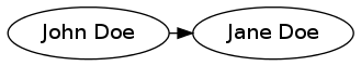In order to lay out the graph, neato uses what is called a ‘spring model’. Imagine all of the nodes of the graphs are weights, and all of the arrows connecting them are compression springs that are trying to push the weights apart. By simulating this process, neato arrives at a figure where the nodes are separated enough to read them, but not so far as to waste space. Now suppose we want to graphically represent the relationship between the main identity in our XML file (i.e., Frank N. Meyer) and all of the identities that he is associated with. We can use a Bash script to build the digraph file automatically from the identity.xml file. We will do this in stages. We start by using the echo command to print out all of the lines of our file. Note we have to use the escape character to include one set of quotation marks inside of another. Use a text editor to create the following file and name it build-digraph.sh

#! /bin/bash

echo "digraph G {"
echo "   \"John Doe\" -> \"Jane Doe\";"
echo "}"

Change the permissions and try executing your shell script with the following commands.

chmod 744 build-digraph.sh
./build-digraph.sh

Instead of echoing the statements inside our digraph, however, we want to construct them using the xmlstarlet bash scripts that we just made. First we input the identity file on the command line and grab the name from it. Use a text editor to edit build-digraph.sh so it now looks as follows.

#! /bin/bash

NAME=$(./get-name.sh $1 | cut -d':' -f2)

echo "digraph G {"
echo "   "${NAME}" -> foobar;"
echo "}"

Try running it with

./build-digraph.sh identity.xml

Now we want to create one line in our digraph file for each associated name. This is clearly a job for the for loop. Use a text editor to edit build-digraph.sh so it now looks as follows.

#! /bin/bash

NAME=$(./get-name.sh $1 | cut -d':' -f2)

echo "digraph G {"
for ANAME in $(./get-assoc-names.sh $1 | cut -d':' -f2)
do
     echo "  "${NAME}" -> "${ANAME}";"
done
echo "}"

To see if it works as expected, try running it with

./build-digraph.sh identity.xml

Your output should look like this:

digraph G {
     "Meyer,FrankNicholas" -> "UnitedStatesDepartmentofAgriculture";
     "Meyer,FrankNicholas" -> "Cunningham,IsabelShipley"; 
     "Meyer,FrankNicholas" -> "UnitedStatesBureauofPlantIndustry";
     "Meyer,FrankNicholas" -> "UnitedStatesOfficeofForeignSeedandPlantIntroduction";
     "Meyer,FrankNicholas" -> "Fairchild,David";
     "Meyer,FrankNicholas" -> "Wilson,ErnestHenry";
     "Meyer,FrankNicholas" -> "PopulationReferenceBureau";
     "Meyer,FrankNicholas" -> "Smith,ErwinF.";
}

That looks good, so we send the output to a .dot file, run it through Graphviz neato and display.

./build-digraph.sh identity.xml > anames.dot
neato -Tpng -Goverlap=false anames.dot > anames.png
display anames.png &

If all went well, the output should look like this:

Trees are graphs, too

Recall that XML files are structured so that tags are properly nested inside one another. We can visualize this containment relationship as a digraph, where we have arrows from outside_tag to inside_tag. In the next section we will use xmlstarlet to extract the structure of our XML file, then Graphviz to plot it in the form of a digraph. Instead of using neato, we will use a different Graphviz plotting routine, dot, which is more appropriate for tree-like figures. Using the -u option, we can eliminate redundant tags when we pull the elements out of an XML file with xmlstarlet el.

xmlstarlet el -u identity.xml | less

Look at the previous listing. In order to convert it into the proper form for Graphviz, we need to turn the forward slashes into arrows. We have a more tricky problem, however. We need to lose everything in a given line except the last two tags and the slash between them. Think about this until you understand why it is the case. We will use grep to pull out the last two tags, separated by a slash. In order to match one or more copies of something that is not a slash, we use the following pattern

([^/]+)

So we want a string of characters that are not a slash, followed by a slash, followed by another string of characters that are not a slash, followed by the end of the line. And we want to match only that (the -o option for extended grep). The following pipeline does what we want.

xmlstarlet el -u identity.xml | grep -E -o '([^/]+)/([^/]+)$' | less

Now we use sed to replace each slash with the correct characters for Graphviz. Our XML tags contain some colons that will be confusing to Graphviz if we leave them in the tags. We are going to translate these into underscores for the purpose of making graph labels. Try the following version of the pipeline.

xmlstarlet el -u identity.xml | grep -E -o '([^/]+)/([^/]+)$' | sed 's/\//->/g' | tr ':' '_' | less

The output looks good, so we can bundle everything into a bash script called build-xml-tree.sh

#! /bin/bash

echo "digraph G {"
for LINK in $(xmlstarlet el -u $1 | grep -E -o '([^/]+)/([^/]+)$' | sed 's/\//->/g' | tr ':' '_')
do
     echo ${LINK}";"
done
echo "}"

Try running the shell script so you can make sure the output looks right.

chmod 744 build-xml-tree.sh
./build-xml-tree.sh identity.xml | less

Finally we lay out our digraph with dot. The -Grankdir option tells Graphviz that we want to use a left-right layout rather than a top-down one. This will give us a figure that is more easily compared with our web browser display.

./build-xml-tree.sh identity.xml > xmltree.dot
dot -Tpng -Goverlap=false -Grankdir=LR xmltree.dot > xmltree.png
display xmltree.png &

The resulting digraph looks like this.

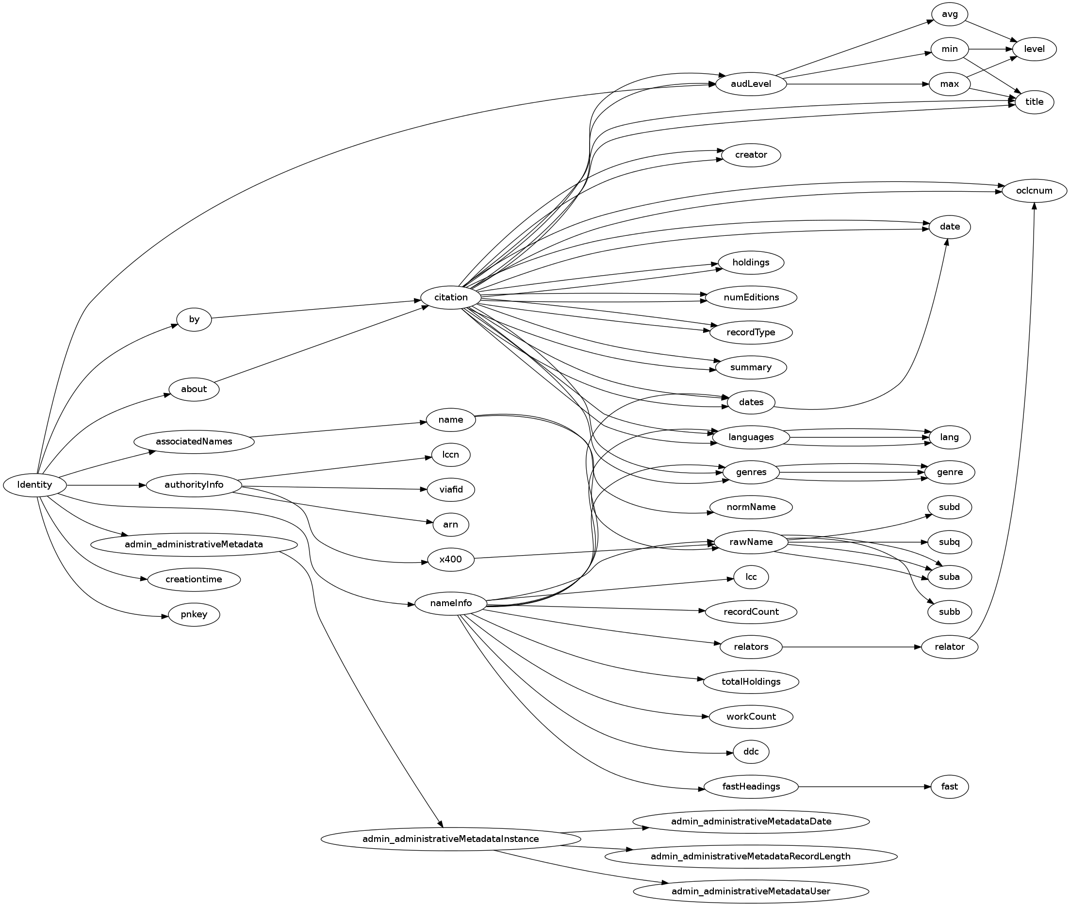
Study this figure for a few minutes. Because it encodes information about the XML file in a different way than the XML display in the web browser does, it makes it easier to see some things. For example, it is obvious when you look at the xmltree.png figure that some tags, like oclcnum or citation, may be children of more than one parent. What else can you discover about the XML file by studying the graph visualization of it?

Introduction

In previous posts we focused on manipulating human- and machine-readible text files that contained prose. Text files are also frequently used to store tabular data or database records that are partially, primarily or completely numeric. Linux and UNIX have a wide variety of commands for manipulating these kinds of files, too. One of the most powerful of these is the Awk programming language, named after its creators Alfred Aho, Peter Weinberger and Brian Kernighan. Awk is standard on Linux and UNIX, and is designed to handle many of the tasks that you might otherwise use a spreadsheet for.

[UPDATE 2014. This post has been modified to reflect changes to the source database since it was originally written. The sense of the original has not been changed. If you are using the HistoryCrawler virtual machine, skip the Installation section and go directly to Downloading a Data Set.]

Installation

We will start by using a web browser to download a data file from an online economic botany database at Kew, the Royal Botanic Gardens. Start your windowing system and open a terminal, then check to see if you have Iceweasel installed. (That is the Debian fork of Firefox; if you are using another Linux distro you will need a web browser of some kind).

man iceweasel

If you don’t get a man page for iceweasel, then install and start it with the following.

sudo aptitude install iceweasel
iceweasel &

We will also be making use of a command line program called csvfix, which is not part of the standard Debian packages. Check to see if it is already installed by typing

csvfix

If you get a “command not found” message, you are going to have to compile the program from source, which requires the Debian build-essential package. Check to see if that is installed with

dpkg -s build-essential | grep Status

If you get a response like “Status: install ok installed”, then you don’t have to install it. Otherwise, use the following to install the build-essential package.

sudo aptitude update
sudo aptitude install build-essential

Now you can download and build the csvfix command with the following:

wget https://bitbucket.org/neilb/csvfix/get/version-1.5.tar.gz
tar -xzvf v*tar.gz
rm v*tar.gz
cd neilb*
make lin
sudo cp ./csvfix/bin/csvfix /usr/local/bin
cd ~

Downloading a data set

Go to the advanced search page of the Economic Botany database at Kew, http://apps.kew.org/ecbot/advancedSearch, and do a search for TDWG Region “China Southeast”. When I did this search I got 278 results, although it is possible the number might increase if new specimens are added to their collection. Click the button labelled “Download Results (CSV)”. This step might take a while. When the data file is ready, your browser will prompt you for a location to save the file. Just put it in your current working directory for now. If you would like to use the exact same data set as I did for this post, you can download a copy here.

Getting an overall sense of the data file

We begin by using some familiar tools to get a sense of what the downloaded file looks like. The file command tells us that there are some Windows CRLF characters in the file, so we make a backup of the original, then use the tr command to create a Linux version of the file with LF characters. The wc command tells us that the file is 305 lines in length and has more than eleven thousand words. (Since the database listed 278 results, why isn’t the file 278 or 279 lines long? This is something that we will definitely want to figure out.) We can use the head command to see that the first line is a listing of fields in our data set. These include things like “Catalogue Number”, “Artefact Name”, and “Expedition”. We save a copy of the field names in search-results-fields.csv. Finally, we can use the tail command to look at the last line in the file and see what a typical record looks like. Note that there are a number of places in this line where we see a string of commas. This tells us that those fields are blank for this particular record. When looking at a structured data set, it is useful to know if or when there may be missing data. We also see that some fields contain numbers (like Catalogue Number: 69603), some contain quote-delimited strings (like Storage Name: “Bottles, boxes etc”) and some contain text that is not in quotes (like Slide: no).

file search-results.csv
mv search-results.csv search-results-bak.csv
cat search-results-bak.csv | tr -d '\r' > search-results.csv
file search-results.csv
wc search-results.csv
head -1 search-results.csv > search-results-fields.csv
cat search-results-fields.csv
tail -1 search-results.csv

Since we have a mixture of textual and numeric data in this file, we can use some of our text analysis tricks to look at things like frequently-occuring words. The pipeline below removes numerals, converts characters to lowercase, changes commas into blank spaces, removes other punctuation, changes blank spaces into newlines, sorts the resulting list of words, compresses repeated instances into a single line and counts them, then sorts the final file in reverse numerical order. Given our search we see some frequent terms we expect to see, like “hong kong”, “chinese” and “china”. We also see that the terms “medicines”, “drugs”, “veterinary”, “medical” and “pharmacies” appear quite frequently, suggesting something about the nature of these botanical samples.

cat search-results.csv | tr -d [:digit:] | tr [:upper:] [:lower:] | tr ',' ' ' | tr -d [:punct:] | tr ' ' '\n' | sort | uniq -c | sort -nr > search-results-frequencies.txt
less search-results-frequencies.txt

When we look at word frequencies, we lose the context in which terms appear. One nice thing about working with structured data is that we can pose and answer numerical or statistical questions. Before we try this, however, we need to have each line in our data file (besides the header) correspond to a single database record.

Fixing spurious line breaks and field separators

We know that the database returned 278 results for our search, and that the first line of our file is a header containing field names. So why doesn’t our file have 279 rows? Let’s hypothesize that the first field, the Catalogue Number, is supposed to be a unique identifier. We can use the cut command to pull out the first column of the data set and have a look at it. The -d option lets us set the delimiter and the -f option lets us specify a field. The first thing we notice is that there is sometimes a quotation mark or line of text in the column, rather than the catalogue number that we are expecting. We use cut again, this time to count the number of lines that don’t contain a digit string. Recall that the -v option for egrep returns lines that do not match the pattern. There are 27 of them. If we subtract 27 (the number of lines that don’t contain a catalogue number) from 305 (the number of lines in the file), we get 278, which is exactly the number of lines we were expecting. It appears as if some of the lines in our data file may have been split into two lines during downloading (with the split usually occurring just before a quotation mark). We can confirm this by using a text editor to have a look at the file. (If you are using HistoryCrawler or another Linux distribution with LibreOffice installed, you can also use Calc to explore the file, but Calc ignores the spurious line breaks when it imports, so you won’t see the problem we are trying to fix.)

cut -d',' -f1 search-results.csv | less
cut -d',' -f1 search-results.csv | egrep -v '^[0-9].+$' | wc -l 

Let’s make a copy of the file where we have removed these spurious line breaks. There are different approaches to a problem like this one, including solutions using awk. Here we will do the following. First we use grep to make sure that our data file doesn’t contain a special character. We’re going to use ‘@’, but it could be any single character that doesn’t occur in the file. Next we change all newlines into this special character, creating a file with one long line. Using the wc command, we confirm that this process hasn’t changed the number of bytes (i.e., characters) in our file. Next we use sed to delete all of the ‘@’ characters that appear just before a non-digit. This sed pattern is complicated by the fact that we want to match any character that isn’t a digit (that is handled by [^0-9]), we need to make a copy of the part of the pattern that we don’t want to delete (which we do by enclosing it in escaped parentheses), and we need to refer back to that copy (which we do with \1). This tutorial explains all of the options we are using. We then can use the wc command to confirm that the resulting file is 26 bytes shorter than the previous one. Finally, we convert all the remaining ‘@’ characters back into newlines, and confirm that the file without spurious line breaks has the right number of lines (i.e., 279 including the header). We clean up by removing temporary files.

grep '@' search-results.csv
wc -c search-results.csv
cat search-results.csv | tr '\n' '@' > search-results-oneline.csv
wc -c search-results-oneline.csv
cat search-results-oneline.csv | sed 's/@\([^0-9]\)/\1/g' > search-results-oneline-edited.csv
wc -c search-results-oneline-edited.csv
cat search-results-oneline-edited.csv | tr '@' '\n' > search-results-edited.csv
wc search-results-edited.csv
rm search-results-oneline*

Now that we have the right number of lines in our data file, we still have a bit of a problem. The comma is used both as a field separator–hence “CSV”, which stands for “comma separated values”–and within individual fields, where it has its usual function as a punctuation mark. If we were to use a simple pattern matching approach to find commas, we would confuse these two different usages. So we need to convert the field separators into a different special character that does not naturally occur in our data. We already know that the ‘@’ is one such character, so we might as well use that for our new field separator.

Sometimes it is possible to use sed, vi or awk to fix a problem like this, but it is pretty easy to make mistakes. Unanticipated special cases can cause problems that are difficult to debug. Instead we will use csvfix to convert our field separators to the ‘@’ character. (See the csvfix manual for more detail about the options used here.) We also use the tail command to make a version of the fixed file that does not contain the first row of field names.

csvfix echo -smq -osep '@' search-results-edited.csv > search-results-fixed.csv
tail -n +2 search-results-fixed.csv > search-results-fixed-noheader.csv

Now we can test our hypothesis that the Catalogue Number field contains unique identifiers. We use cut in a pipeline to show that each Catalogue Number appears only once.

cut -d'@' -f1 search-results-fixed.csv | sort -n | uniq -c | less

Answering questions about the data

When we wanted to select the first column of data, we used the -f1 option for cut. It will be handy to have a list of column numbers and headings, so we make a file containing those. Now we know, for example, that if we want to see which plant parts are held for a particular specimen, we need to look at the 33rd field (column).

cat search-results-fields.csv | tr ',' '\n' | cat -n > search-results-field-nums.txt
less search-results-field-nums.txt

How many different kinds of plant parts are represented in this data set, and how many of each kind are there? We can use a familiar pipeline to find out, as shown in the next example. We see that wood is the most common kind of specimen (76 cases), that 47 of the records have no indication of what kind of plant matter has been collected, that 37 specimens are seeds, 32 are fruits, 30 are roots, and so on.

cut -d'@' -f33 search-results-fixed-noheader.csv | sort | uniq -c | sort -nr

Field 6, the Artefact Name, contains a more detailed description of each specimen.

cut -d'@' -f6 search-results-fixed-noheader.csv | sort | uniq -c | sort -nr | less

Here we see that a lot of the specimens are listed as CHINESE DRUGS of various kinds. We can modify the command above to pull out those records:

cut -d'@' -f6 search-results-fixed-noheader.csv | sort | uniq -c | sort -nr | grep 'CHINESE DRUGS' | less

If we want to count the number of items listed as CHINESE DRUGS, we could do it with a command like this:

cut -d'@' -f6 search-results-fixed-noheader.csv | grep 'CHINESE DRUGS' | wc -l

Answering more complicated queries with Awk programs

Often we are interested in answering questions that draw on information stored across multiple fields. For example, how many of the specimens listed as CHINESE DRUGS don’t come from Hong Kong? To answer this, we will also need to draw on information from field 13, TDWG Region. This is a good opportunity to build up an example Awk program step-by-step.

First we need to pull out the fields of interest. Instead of using cut, we can do this with awk. We use the -F option to indicate our field separator, and enclose the Awk program in single quotes. The curly braces tell awk to print the thirteenth and sixth fields for every line of the input file. We put a tab between the fields to make it easier to see where one ends and the next begins.

awk -F'@' '{ print $13, "\t", $6 }' search-results-fixed-noheader.csv

We can modify the program so that it only prints lines that match a particular pattern. In this case, we are only interested in the lines where field 6 matches ‘CHINESE DRUGS’.

awk -F'@' '$6 ~ /CHINESE DRUGS/ { print $13, "\t", $6 }' search-results-fixed-noheader.csv

And of those, we only want to see the lines where field 13 does not match ‘Hong Kong’. The double ampersand means that both patterns have to be satisfied for the action to occur.

awk -F'@' '$13 !~ /Hong Kong/ && $6 ~ /CHINESE DRUGS/ { print $13, "\t", $6 }' search-results-fixed-noheader.csv

Here is another example using Awk. In field 34, TDWG Use, we see that some of the specimens are listed as FOOD, MATERIALS, MEDICINES, POISONS or some combination thereof. We will write a short program to count the number of each. We start by counting the instances labeled as FOOD. Note that we create a variable to hold the count. This variable is incremented by 1 for each record where field 34 matches ‘FOOD’. When the program is finished going through our file line-by-line, we print the resulting sum.

awk -F'@' '$34 ~ /FOOD/ { foodsum++ } END { print "Food ", foodsum } ' search-results-fixed-noheader.csv

We need a separate variable to keep track of the count of each of the labels we are interested in. Here is how we modify the program to count lines that match ‘MATERIALS’, too.

awk -F'@' '$34 ~ /FOOD/ { foodsum++ } $34 ~ /MATERIALS/ { matsum++ } END { print "Food ", foodsum; print "Materials " matsum } ' search-results-fixed-noheader.csv

Putting the entire program on one line like this can quickly get complicated. Instead we will use a text editor to edit and save the program in a file called count-labels. Note that we are setting the field separator inside our program now, rather than as an option when we call awk.

#! /usr/bin/awk -f
BEGIN {
     FS="@"
}
$34 ~ /FOOD/ { foodsum++ }
$34 ~ /MATERIALS/ { matsum++ }
END {
     print "Food ", foodsum;
     print "Materials ", matsum
}

Then we can change the permissions and run the program with

chmod 744 count-labels
./count-labels search-results-fixed-noheader.csv

Now we can add the other labels to the program and try running it again.

#! /usr/bin/awk -f
BEGIN {
     FS="@"
}
$34 ~ /FOOD/ { foodsum++ }
$34 ~ /MATERIALS/ { matsum++ }
$34 ~ /MEDICINES/ { medsum++ }
$34 ~ /POISONS/ { poisonsum++ }
END {
     print "Food ", foodsum
     print "Materials ", matsum
     print "Medicines ", medsum
     print "Poisons ", poisonsum
}

We see that 113 of the specimens have medicinal uses, whereas only two are listed as poisons. Try writing an Awk program to list the samples that were donated before 1920, using the Donor Date field.

Introduction

We have already seen that the default assumption in Linux and UNIX is that everything is a file, ideally one that consists of human- and machine-readable text. As a result, we have a very wide variety of powerful tools for manipulating and analyzing text files. So it makes sense to try to convert our sources into text files whenever possible. In the previous post we used optical character recognition (OCR) to convert pictures of text into text files. Here we will use command line tools to extract text, images, page images and full pages from Adobe Acrobat PDF files.

Installation

[UPDATE 2014. If you are working with the HistoryCrawler virtual machine, the KDE GUI and PDF tools are already installed. Skip to the next section.]

Since we will be working with pictures of text as well as raw text files, we need to use a window manager or desktop environment. Start your windowing system and open a terminal. I assume that you already have Tesseract OCR and ImageMagick installed from the previous lesson. Now we need to install tools for working with Adobe Acrobat PDF documents. Try

man xpdf
man pdftk
man pdftotext

If you don’t get a man page for xpdf, then install it with the following.

sudo aptitude install xpdf

If you don’t get a man page for pdftk, then install it.

sudo aptitude install pdftk

If you don’t get a man page for pdftotext, then install the Poppler Utilities with the following command. This package includes a number of useful tools. The apropos command shows all of the tools that we now have at our disposal for manipulating PDF files.

sudo aptitude install poppler-utils
apropos pdf | less

Viewing PDFs

Adobe’s portable document format (PDF) is an open standard file format for representing documents. Although PDFs can (and often do) contain text, they are not easily read using Linux commands like cat, less or vi. Instead you need to use a dedicated reader program to view PDFs, or command-line tools to extract information from them.

Let’s start by downloading a PDF to work with. We will be using a 1923 book about the wildflowers of Kashmir from the Internet Archive.

wget http://archive.org/download/WildFlowersOfKashmir/KashmirWildflowers.pdf

[UPDATE 2014. If you are using HistoryCrawler, you can view the PDF with Okular. The ampersand runs the process in the background, allowing you to continue using your terminal while looking at the PDF.

okular K*pdf &

Spend some time getting to know the capabilities of Okular, then skip ahead to the next section.]

If you don’t have a GUI, you can view this document using xpdf. Try searching for a word, say ‘China’, using the binoculars icon. You may have to enlarge the xpdf window a bit to see all the icons at the bottom. Note that we are also running the process in the background (using the ampersand on the command line) so we can continue to use our terminal while viewing PDFs. When you use the mouse to close the xpdf window, it kills the process. You could also use the kill command from the terminal to close it.

xpdf K*pdf &

Extracting text

The pdftotext command allows us to extract text from an entire PDF or from a particular page range. We start by grabbing all of the text from our document, then using the less command to have a look at it. If a document is born digital–that is, if the PDF is created from electronic text in another application, like a word processor or email program–then the text that is extracted should be reasonably clean. If it is the product of OCR, however, then it will probably be messy, as it is here. We can, of course, use all of the command-line tools that we have already covered to manipulate and analyze the KashmirWildflowers.txt file.

pdftotext KashmirWildflowers.pdf KashmirWildflowers.txt
less KashmirWildflowers.txt
egrep -n --color China KashmirWildflowers.txt

Extracting page images and creating a contact sheet

This source contains a number of photographs, and we can extract these using the pdfimages command. By default, black and white images are stored as a Portable Bitmap (pbm) file, and colour ones as a Portable Pixmap (ppm) file. When you use ImageMagick display to view these files, they show up as white on black unless you use the -negate option.

mkdir images
pdfimages KashmirWildflowers.pdf images/KashmirWildflowers
ls images
display -negate images/KashmirWildflowers-025.pbm &

If you spend some time exploring the image files in the images directory, you will notice that many of them are pictures of text rather than flower photographs. This is to be expected in an OCRed document, because each text page starts as a picture of text. It would be nice to see all of the images at once, so we could figure out which ones actually are pictures of flowers. If we were using a graphical file browser like the Mac Finder or Windows File Explorer, we would be able to look through thumbnails and drag and drop the files into different directories. (Linux GUI desktops like KDE also have a lot of options for graphical file browsing, if you want to go this route.) Instead, we are going to use ImageMagick to make a ‘contact sheet’, a single image comprised of thumbnails of the first hundred image files in the images directory.

montage -verbose -label '%f' -define pbm:size=200x200 -geometry 100x100+38+6 -tile 5x images/*0??.pbm[100x100] images-contact.jpg
display images-contact.jpg &

In the command above, we use the -verbose option to tell ImageMagick that we want feedback on what it is doing. The -label option says each thumbnail should be labeled with its filename. We resize the incoming images with the -define option and with the stuff in square brackets appended to the source filename pattern. (This is so we don’t run the risk of running out of memory by storing lots of huge pictures during processing). The -geometry option tells ImageMagick to output thumbnails of 100 by 100 pixels, with some room around each to include the caption. The -tile option says to put the output in 5 columns, and as many rows as necessary. We use wildcards to specify the first hundred images. Once we have created our contact sheet, we can view it with display.

Iterating through an array

Now we want to copy the flower images in the first hundred pages to a new directory. We could type out one mv command for each file, but that would be pretty tedious. Instead we are going to store the numbers of the files that we want to move in an array, then use a bash for loop to step through the array and move each file.

We start by storing the file numbers

filenums=(025 028 032 035 038 040 043 046 050 054 057 060 062 065 069 073 077 080 082 085 088 091 094 096 098)

The next step is to loop through each element of the array and create a full filename from it. We want to test this part of the process before using it in a command, so we simply echo each filename to the terminal.

for num in ${filenums[@]} ; do echo images/KashmirWildflowers-${num}.pbm ; done

That looks good. Make sure you are in the directory that contains KashmirWildflowers.pdf and then modify the for loop to copy the flower images to a new directory, as shown below. When we finish, we make a new contact sheet of the flower images.

mkdir flowerimages
for num in ${filenums[@]} ; do cp images/KashmirWildflowers-${num}.pbm flowerimages/ ; done
ls flowerimages
montage -verbose -label '%f' -define pbm:size=200x200 -geometry 100x100+38+6 -tile 5x flowerimages/*.pbm[100x100] flowerimages-contact.jpg
display flowerimages-contact.jpg &

The contact sheet of all the flower images in the book looks like this:

The image with flowers from the first hundred pages is about half as long.

An alternative workflow would be to use Okular or xpdf to identify the pages for each flower picture, and then use the -f and -l options for pdfimages to extract just the page images we are interested in. Experiment with this approach.

Compiling individual image files into a new PDF

If we have a collection of image files in a directory, we can compile them into a new PDF using the ImageMagick convert command. Here we use the -negate option so the final result is black on white instead of inverted.

convert -negate flowerimages/*.pbm flowerimages.pdf

View the output with Okular or xpdf. The same technique could be used, for example, to aggregate all of the photographs taken during a day of archival work or fieldwork into a single PDF.

Manipulating PDFs with pdftk

The pdftk command gives us a variety of options for manipulating PDFs. Here are a few examples. After trying each one, use Okular or xpdf to see the results.

The third page of KashmirWildflowers.pdf is a photograph of Dal Lake. In the original publication it was rotated so that it would fit better when printing, but for onscreen use we might prefer to have it the right way up. The command below extracts the page and rotates it ninety degrees clockwise.

pdftk KashmirWildflowers.pdf cat 3east output KashmirWildflowers-p003-rotated.pdf

Pages 230-233 of the original document contain a general index. We can extract just these pages into a separate PDF with the following command.

pdftk KashmirWildflowers.pdf cat 230-233 output KashmirWildflowers-pp230-233-index.pdf

The pdftk command gives us a way to extract metadata from PDFs, too. We can also access the same information with the pdfinfo command. Using the commands below, we can see that our original PDF has a number of associated key-value pairs.

pdftk KashmirWildflowers.pdf dump_data | less
pdfinfo KashmirWildflowers.pdf

The key Creator, for example, is associated with the value Adobe Scan-to-PDF Utility 4.0, and the CreationDate was Feb 2, 2012 around three-thirty in the afternoon. If you run the following commands, you should find that the Creator and CreationDate are different for a file that you just created.

pdftk KashmirWildflowers-pp230-233-index.pdf dump_data
pdfinfo KashmirWildflowers-pp230-233-index.pdf

Bursting a PDF

In a previous post, we burst a long document into separate pages before indexing it with a search engine. We did this so that searches would result in more fine-grained matches rather than simply telling us that the whole document was somehow relevant. The pdftk command allows us to burst a PDF into single pages, and at the same time outputs file metadata to a file called doc_data.txt.

pdftk KashmirWildflowers.pdf burst
less doc_data.txt
mkdir docpages
mv pg*pdf docpages

View the third page to check your work, using

xpdf docpages/pg_0003.pdf &

or

okular docpages/pg_0003.pdf &

Then …

pdftotext docpages/pg_0006.pdf KashmirWildflowers-p006.txt
less KashmirWildflowers-p006.txt

Adding metadata

Using pdftk, it is also possible to add metadata to a PDF, and even to attach other files to it. We start by using vi, atom or another file editor to create a file called KashmirWildflowers-metadata.txt containing the following information.

InfoKey: Title
InfoValue: Wild Flowers of Kashmir
InfoKey: Author
InfoValue: Coventry, B. O.
InfoKey: Keywords
InfoValue: London,1923,Raithby Lawrence and Company

Next, we update the PDF to contain this new information, then check our work. Note that the modification date metadata does not change automatically; we would have to do this explicitly if we wanted it changed.

pdftk KashmirWildflowers.pdf update_info KashmirWildflowers-metadata.txt output KashmirWildflowers-updated.pdf
pdftk KashmirWildflowers-updated.pdf dump_data
pdfinfo KashmirWildflowers-updated.pdf

We can attach files to a PDF and extract them again using the attach_files and unpack_files options of pdftk (see the man page for more details). The xdpf viewer shows attachments with a pushpin icon, but it does not let us inspect the attached files. Experiment with this if you are curious, but we won’t make use of the file attachment capability right now.

Introduction

In previous posts, we looked at a variety of Linux command line techniques for analyzing text and finding patterns in it, including word frequencies, permuted term indexes, regular expressions, simple search engines and named entity recognition. In this post we focus on a preliminary issue: converting images of texts into text files that we can work with. Starting with digital photographs or scans of documents, we can apply optical character recognition (OCR) to create machine-readable texts. These will certainly have some errors, but the quality tends to be surprisingly good for clean scans of recently typed or printed pages. Older fonts and texts, or warped, indistinct or blurry page images often result in lower quality OCR.

Using a window manager

As with earlier posts, we are going to use command line tools to process our files. When working with page images, however, it is very useful to be able to see pictures. The standard Linux console does not have this facility, so we need to use a window manager or a GUI desktop environment. The former is a lightweight application that allows you to view and manipulate multiple windows at the same time; the latter is a full-blown interface to your operating system that includes graphical versions of your applications. Sometimes you use a mouse with a window manager, but most of your interactions continue to be at the command line. With a GUI desktop, the expectation is that you will spend most of your time using a mouse for interaction (this is very familiar to users of Windows or OS X). In Linux, you can choose from a variety of window managers and desktop environments.

[UPDATE 2014. If you are using the HistoryCrawler virtual machine, you already have the KDE GUI installed. Skip the “Installation” section and go directly to “Viewing Images of Text”.]

Installation

If you are working with a Linux distribution that does not already have a windowing manager or desktop environment installed, you will need one. Here I will be using a window manager called Openbox, but most of the commands should work fine with other Linux configurations. Try

man startx

If you don’t get a man page, you can install X Windows and Openbox with the following.

sudo aptitude install xorg xserver-xorg xterm
sudo aptitude install openbox obconf obmenu

Next we will want some command-line image processing software to manipulate page images. Check to see if ImageMagick is installed with

man imagemagick

If you don’t get a man page, install it with

sudo aptitude install imagemagick

We will install three other utilities for working with files: zip / unzip, pandoc and tre-agrep. Check for man pages…

man zip
man pandoc
man tre-agrep

… and install if necessary.

sudo aptitude install zip unzip
sudo aptitude install pandoc
sudo aptitude install tre-agrep

Finally, we want to install Tesseract, the program which performs the OCR. Check to see if it is already installed with

man tesseract

If not, install with the following commands

sudo aptitude install tesseract-ocr tesseract-ocr-eng

Note that I am only installing the English language OCR package here. If you want to install additional natural languages, see the Tesseract web site for further instructions.

We start our windowing manager with

startx

Once it is running the background will turn dark grey and you will see a mouse pointer. Right click on the mouse to get a menu and choose “Terminal emulator”. This will give us the terminal that we will use for our commands.

Viewing images of text

The source that we will be working with is the same one that we used in the previous post. It is a collection of scanned correspondence between Frank N. Meyer and his superior at the US Department of Agriculture, relating to an expedition to South China between 1916 and 1918. We start by making a directory for the source and downloading XML metadata, OCRed text and a zipped directory of page images (in JPEG 2000 format). This will take a few minutes to complete.

mkdir meyer
cd meyer
wget -r -H -nc -nd -np -nH --cut-dirs=2 -e robots=off -l1 -A .xml,.txt,.zip 'http://archive.org/download/CAT10662165MeyerSouthChinaExplorations/'

Next we unzip the directory of page images and remove the zipped file.

unzip CAT*zip
rm CAT*zip
mv CAT31091908_jp2 jp2files

Let’s take the hundredth page of our source as a sample image to work with. We can look at the JPEG 2000 image of the page using the ImageMagick display command. Since the image is very high resolution, we scale it to 25% of the original size and even then we can only see a small amount of it in the window. We have to scroll around with the mouse to look at it. Click the X in the upper right hand corner of the display window to dismiss it. Note that since we don’t want to tie up our terminal while the display command is operating, we run it in the background by adding an ampersand to the command line.

cp jp2files/CAT31091908_0100.jp2 samplepg.jp2
display -geometry 25%x25% samplepg.jp2 &

We can create a smaller version of the page image with the ImageMagick convert command. This version is much easier to read on screen.

convert samplepg.jp2 -resize 25% samplepg-25.jpg
display samplepg-25.jpg &

Optical character recognition

We can open the OCRed text from the Internet Archive with

less CAT31091908_djvu.txt

Use /49 and n in the less display to search for the page in question. Note how good the OCR is on the first part of that page, confusing only the 2 and comma in the date “June 29, 1917”. Skipping ahead, we see a few other errors: “T realize” for “I realize”, “v/hat” for “what”, and the like. For convenience, let’s yank the OCRed text out of the file to a separate file. We use less -N to find the line numbers of the beginning and end of the OCRed page.

less -N CAT31091908_djvu.txt
cat CAT31091908_djvu.txt | sed '5837,5896!d' > samplepg_djvu.txt
less samplepg_djvu.txt

Since we already have a good text file for this document, we don’t really need to do OCR on the page images. If we did not have the text, however, we could create our own with Tesseract. Since Tesseract does not work with JPEG 2000 images, we first use ImageMagick to create a greyscale TIF file. Try the following commands.

convert samplepg.jp2 -colorspace Gray samplepg-gray100.tif
tesseract samplepg-gray100.tif samplepg_tesseract
less samplepg_tesseract.txt

Note that this OCR is really good, too, and that the few errors that occurred are different than the ones in the DJVU OCR. We can use the diff command to find the parts of the two OCR files that do not overlap. The options which we provide to diff here cause it to ignore blank lines and whitespace, and to report only on those lines which differ from one file to the next. You can learn more about the output of the diff command by consulting its man page.

diff -b -B -w --suppress-common-lines samplepg_djvu.txt samplepg_tesseract.txt | less

A trickier case for OCR

A clean, high resolution scan of a page of printed text is the best-case scenario for OCR. If you do archival work, you may have a lot of digital photos of documents that are rotated, warped, unevenly lit, blurry, or partially obscured by fingers. The documents themselves may be photocopies, mimeograph pages, dot-matrix printouts, or something even more obscure. In cases like these, you have to decide how much time you want to spend cleaning up your page images. If you have a hundred of them, and each is very important to your project, it is worth doing it right. If you have a hundred thousand and you just want to mine them for interesting patterns, something quicker and dirtier will have to suffice.

As an example of a more difficult OCR job, consider this newspaper article about Meyer’s expedition from the Tacoma Times (15 Feb 1910). This comes from the Library of Congress Chronicling America project, a digital archive of historic newspapers that provides JPEG 2000, PDF and OCR text files for every page, neatly laid out in a directory structure that is optimized for automatic processing.

First we download the image and OCR text. When we ask for the latter, we will actually get an HTML page, so we use pandoc to convert that to text. Then we use sed to extract the part of the OCR text that corresponds to our article, and use less to display it. We see that the supplied OCR is pretty rough, but probably contains enough recognizable keywords to be useful for search (e.g., “persimmon”, “Meyer”, “China”, “Taft”, “radishes”, “cabbages”, “kaki”).

wget http://chroniclingamerica.loc.gov/lccn/sn88085187/1910-02-15/ed-1/seq-4.jp2 -O tacoma.jp2
wget http://chroniclingamerica.loc.gov/lccn/sn88085187/1910-02-15/ed-1/seq-4/ocr/ -O tacoma-lococr.html
pandoc -o tacoma-lococr.txt tacoma-lococr.html
cat tacoma-lococr.txt | sed '117,244!d' | sed '55,102d' | tr -d '\\' > tacoma-meyer-lococr.txt
less tacoma-meyer-lococr.txt

Before trying to display the JPEG 2000 file, we use the ImageMagick identify command to learn more about it. We see that it is 5362×6862 pixels and 4.6MB in size. That is too big for us to look at easily, but we can use ImageMagick to make a small JPG copy to display.

identify tacoma.jp2
convert tacoma.jp2 -resize 10% tacoma-10.jpg
display tacoma-10.jpg

The Chronicling America site already provides OCR text which is usable for some tasks. It’s not clear if we can do a better job or not. If we wanted to try, we would start by using ImageMagick to extract the region of the JPEG 2000 image that contains the Meyer article, then use Tesseract on that. The sequence of commands below does exactly this. It is not intended to be tutorial, but rather to suggest how one might use command line tools to begin to figure out a workflow for dealing with tricky OCR cases. In this case, the Tesseract output is not really better than the OCR supplied with the source, although it might be possible to get better results with more image processing. If you find yourself using ImageMagick a lot for this kind of work, you might be interested in the textcleaner script from Fred’s ImageMagick Scripts.

convert -extract 2393x3159+0+4275 tacoma.jp2 tacoma-extract.jp2
convert -extract 1370x2080+100+200 tacoma-extract.jp2 tacoma-meyer.jp2
display tacoma-meyer.jp2 &
convert tacoma-meyer.jp2 tacoma-meyer.tif
tesseract tacoma-meyer.tif tacoma-meyer-tesocr
less tacoma-meyer-tesocr.txt

Assessing OCR quality

Let’s return to the Meyer correspondence. We have an OCR file for the whole document, CAT31091908_djvu.txt. Using techniques that we covered in previous posts, we can create a word list…

cat CAT31091908_djvu.txt | tr [:upper:] [:lower:] | tr -d [:punct:] | tr -d [:digit:] | tr ' ' '\n' | sort > CAT31091908_djvu-allwords.txt
uniq CAT31091908_djvu-allwords.txt > CAT31091908_djvu-wordlist.txt
less CAT31091908_djvu-wordlist.txt

… then determine word frequencies and look through them to figure out what the text might be about. We find “letter”, “meyer”, “china”, “pear”, “species”, “seed”, “reimer”, “chinese”, “seeds” and “plants”.

uniq -c CAT31091908_djvu-allwords.txt | sort -n -r > CAT31091908_djvu-wordfreqs.txt
less CAT31091908_djvu-wordfreqs.txt

We can also find all of the non-dictionary words in our OCR text and study that list to learn more about the errors that may have been introduced.

fgrep -i -v -w -f /usr/share/dict/american-english CAT31091908_djvu-wordlist.txt > CAT31091908_djvu-nondictwords.txt
less CAT31091908_djvu-nondictwords.txt

We see things that look like prefixes and suffixes: “agri”, “ameri”, “alities”, “ation”. This suggests we might want to do something more sophisticated with hyphenation. We see words that may be specialized vocabulary, rather than OCR errors: “amaranthus”, “amygdalus”, “beancheese”. We also see variants of terms which clearly are OCR errors: “amydalus”, “amykdalus”, “amypdalu”.

Approximate pattern matching

When we used pattern matching in the past, we looked for exact matches. But it would be difficult to come up with regular expressions to match the range of possible OCR errors (or spelling mistakes) that we might find in our sources. In a case like this we want to use fuzzy or approximate pattern matching. The tre-agrep command lets us find items that sort of match a pattern. That is, they match a pattern up to some specified number of insertions, deletions and substitutions. We can see this in action by gradually making our match fuzzier and fuzzier. Try the commands below.

tre-agrep -2 --color amygdalus CAT31091908_djvu.txt
tre-agrep -4 --color amygdalus CAT31091908_djvu.txt

With two possible errors, we see matches for “Pyrus amgydali folia”, “AmyKdalus”, “Mnygdalus”, “itoygdalus”, “Araugdalus” and “Amy^dalus”. When we increase the number of possible errors to four, we see more OCR errors (like “Amy^dalus”) but we also begin to get a lot of false positives that span words (with the matches shown here between square brackets): “I [am als]o”, “m[any days]”, “pyr[amidal f]orm”, “orn[amental s]tock”, “hills [and dales]”. If it helps, you can think of fuzzy matching as a signal detection problem: we want to maximize the number of hits while minimizing the number of false positives.

Introduction

In earlier posts we used a variety of tools to locate and contextualize words and phrases in texts, including regular expressions, concordances and search engines. In every case, however, we had to have some idea of what we were looking for. This can be a problem in exploratory research, because you usually don’t know what you don’t know. Of course it is always possible to read or skim through moderate amounts of text, but that approach doesn’t scale up to massive amounts of text. In any event, our goal is to save our care and attention for the tasks that actually require it, and to use the computer for everything else. In this post we will be using named entity recognition software from the Stanford Natural Language Processing group to automatically find people, places and organizations mentioned in a text.

In this post, we are going to be working with a book-length collection of correspondence from the Internet Archive. The digital text was created with optical character recognition (OCR) rather than being entered by hand, so there will be a number of errors in it. Download the file.

wget http://archive.org/download/CAT10662165MeyerSouthChinaExplorations/CAT31091908_djvu.txt

Installation

The recognizer is written in Java, so we need to make sure that is installed first. Try

man java

If you don’t get a man page in return, install the Java runtime and development kits.

sudo aptitude update
sudo aptitude upgrade
sudo aptitude install default-jre default-jdk

Confirm that you have Java version 1.6 or greater with

java -version

You will also need utilities for working with zipped files. Try

man unzip

If you don’t get a man page, you will need to install the following.

sudo aptitude install zip unzip

Now you can download the named entity recognition software. The version that I installed was 3.2.0 (June 20, 2013). If a newer version is available, you will have to make slight adjustments to the following commands

wget http://nlp.stanford.edu/software/stanford-ner-2013-06-20.zip
unzip stanford*.zip
rm stanford*.zip
mv stanford* stanford-ner

[UPDATE 2104. If you are using the HistoryCrawler VM, Stanford NER is already installed in your home directory. You can copy it to your current working directory with the following command.]

cp -r ~/stanford-ner .

Labeling named entities

Now we can run the named entity recognizer on our text. The software goes through every word in our text and tries to figure out if it is a person, organization or location. If it thinks it is a member of one of those categories, it will append a /PERSON, /ORGANIZATION or /LOCATION tag respectively. Otherwise, it appends a /O tag. (Note that this is an uppercase letter O, not a zero). There are more than 80,000 words in our text, so this takes a few minutes.

stanford-ner/ner.sh CAT31091908_djvu.txt > CAT31091908_djvu_ner.txt

Spend some time looking at the labelled text with

less CAT31091908_djvu_ner.txt

Our next step is to create a cleaner version of the labeled file by removing the /O tags. Recall that the sed command ‘s/before/after/g’ changes all instances of the before pattern to the after pattern. The pattern that we are trying to match has a forward slash in it, so we have to precede that with a backslash to escape it. We don’t want to match the capital O in the /ORGANIZATION tag, either, so we have to be careful to specify the blank spaces in both before and after patterns. The statement that we want looks like this

sed 's/\/O / /g' < CAT31091908_djvu_ner.txt > CAT31091908_djvu_ner_clean.txt

You can use less to confirm that we removed the /O tags but left the other ones untouched.

Matching person tags

Next we will use regular expressions to create a list of persons mentioned in the text (and recognized as such by our named entity recognizer). The recognizer is by no means perfect: it will miss some people and misclassify some words as personal names. Our text is also full of spelling and formatting errors that are a result of the OCR process. Nevertheless, we will see that the results are surprisingly useful.

The regular expression that we need to match persons is going to be complicated, so we will build it up in a series of stages. We start by creating an alias for egrep

alias egrepmatch='egrep --color -f pattr'

and we create a file called pattr that contains

Meyer

Now when we run

egrepmatch C*clean.txt

we see all of the places in our text where the name Meyer appears. But we also want to match the tag itself, so we edit pattr so it contains the following and rerun our egrepmatch command.

Meyer/PERSON

That doesn’t match any name except Meyer. Let’s change pattr to use character classes to match all the other personal names. Re-run the egrepmatch command each time you change pattr.

[[:alpha:]]*/PERSON

That is better, but it is missing the middle initial in forms like Frank N. Meyer. So we have to say we want to match either alphabetical characters or a period. Now pattr looks like the following. (Because the period is a special character in regular expressions we have to escape it with a backslash.)

([[:alpha:]]|\.)*/PERSON

That looks pretty good. The next problem is a bit more subtle. If we stick with the pattern that we have now, it is going to treat Henry/PERSON Hicks/PERSON as two separate person names, rather than grouping them together. What we need to capture is the idea that a string of words tagged with /PERSON are clumped together to form a larger unit. First we modify pattr so that each matching term is followed either by whitespace or by an end of line character.

([[:alpha:]]|\.)*/PERSON([[:space:]]|$)

The last step is to indicate that one or more of these words tagged with /PERSON makes up a personal name. Our final pattern is as follows.

(([[:alpha:]]|\.)*/PERSON([[:space:]]|$))+

Copy this file to a new file called personpattr.

Extracting a list of personal names and counting them

To make a list of persons in our text, we run egrep with the -o option, which omits everything except the matching pattern. Run the following command and then explore CAT31091908_djvu_ner_pers.txt with less. Note that it includes names like David Fairchild and E. E. Wilson, which is what we wanted.

egrep -o -f personpattr CAT31091908_djvu_ner_clean.txt > CAT31091908_djvu_ner_pers.txt

Next we use a familiar pipeline to create frequency counts for each person labeled in our text.

cat CAT31091908_djvu_ner_pers.txt | sed 's/\/PERSON//g' | sort | uniq -c | sort -nr > CAT31091908_djvu_ner_pers_freq.txt

When we use less to explore this frequency file, we find some things of interest. During OCR, the letter F was frequently mistaken for P (there are about the same number of Pairchilds and Fairchilds, for example, as well as four Prank Meyers.) We also see a number of words which will turn out not to be personal names on closer inspection. Brassica and Pistacia are plant genera, Iris Gardens is likely a place, N. W. of Hsing a direction and S. S. Feng Yang Maru the name of a vessel. But these errors are interesting, in the sense that they give us a bit better idea of what this text might be about. We also see different name forms for the same individual: Meyer, Frank Meyer and Frank N. Meyer, as well OCR errors for each.

Given a set of names, even a noisy one like this, we can begin to refine and automate our process of using the information that we have to find new sources that may be of interest. The second most common name in our text is Reimer. A quick Google search for “frank meyer” reimer turns up new sources that are very relevant to the text that we have, as do searches for “frank meyer” swingle, “frank meyer” wilson, and “feng yang maru”.

Organization and location names

The recognizer also tagged words in our text that appeared to be the names of organizations or locations. These labels are not perfect either, but they are similarly useful. To extract a list of the organization names and count the frequency of each, create a file called orgpattr containing the following regular expression.

(([[:alnum:]]|\.)+/ORGANIZATION([[:space:]]|$))+

Then run these commands.

egrep -o -f orgpattr CAT31091908_djvu_ner_clean.txt > CAT31091908_djvu_ner_org.txt
cat CAT31091908_djvu_ner_org.txt | sed 's/\/ORGANIZATION//g' | sort | uniq -c | sort -nr > CAT31091908_djvu_ner_org_freq.txt

To pull out locations, create a file called locpattr containing the following regular expression. (Note that place names are often separated by commas, as in Chihli Prov., China.)

(([[:alnum:]]|\.)+/LOCATION[[:space:]](,[[:space:]])?)+

Then run these commands.

egrep -o -f locpattr CAT31091908_djvu_ner_clean.txt > CAT31091908_djvu_ner_loc.txt
cat CAT31091908_djvu_ner_loc.txt | sed 's/\/LOCATION//g' | sort | uniq -c | sort -nr > CAT31091908_djvu_ner_loc_freq.txt

Use less to explore both of the new frequency files. The location file has trailing commas and spaces, which are throwing off the frequency counts. Can you figure out how to modify the pipeline and or regular expression to fix this?

Google searches for new terms like “frank meier” hupeh and “yokohama nursery company” continue to turn up relevant new sources. Later we will learn how to automate the process of using named entities to spider for new sources.

Introduction

In previous posts we downloaded a single book from the Internet Archive, calculated word frequencies, searched through it with regular expressions, and created a permuted term index. In this post, we extend our command line methods to include automatically downloading an arbitrarily large batch of files and building a simple search engine for our collection of sources.

In order to download a batch of files from the Internet Archive, we need a search term that will work on the advanced search page of the site. For the example here, I am going to be using the search

collection:gutenberg AND subject:"Natural history -- Juvenile literature"

There is a very nice post on the Internet Archive blog explaining the process in detail for a Mac or Windows machine. Here we will do everything at the Linux command line. For our trial we will only be using a few books, but the same method works just as well for hundreds or thousands of sources.

[UPDATE 2014. Because the subject categories at the Internet Archive were changed for one of the books since this post was written, I have had to make a few minor edits below. These do not change the sense of the original lesson.]

URL Encoding and the HTTP GET Method

First, a quick review of URL encoding and the HTTP GET method. Files on a web server are are stored in a nested directory structure that is similar to the Linux / UNIX filesystem. To request a file, you have to give your web browser (or a program like wget) a URL, or uniform resource locator. Think of this like the address of a file. It starts with a message telling the server what protocol you want to use to communicate (e.g., HTTP). This is followed by the name of the host (typically a domain name like archive.org), an optional port number (which we don’t need to deal with here) and then the path to the resource you want. If the resource is a file sitting in a directory, the path will look a lot like a file path in Linux. For example,

https://github.com/williamjturkel/Digital-Research-Methods/blob/master/README.md

For many sites, however, it is possible to send a custom query to the web server and receive some content as a result. One way of doing this is with the HTTP GET method. Your file path includes a query string like

?lastname=Andrews&firstname=Jane

and the server responds appropriately. (The exact query that you send will depend on the particular web server that you are contacting.)

Regardless of whether you are requesting a single file or sending an HTTP GET, there has to be a way of dealing with blank spaces, punctuation and other funky characters in the URL. This is handled by URL encoding, which converts the URL into a form which can be readily sent online.

When it is URL encoded, the query string that we are going to send to the Internet Archive

collection:gutenberg AND subject:"Natural history -- Juvenile literature"

becomes something like

collection%3Agutenberg%20AND%20subject%3A%22Natural+history+--+Juvenile+literature%22

or

collection%3Agutenberg+AND+subject%3A%22Natural+history+--+Juvenile+literature%22

We will see one way to do this URL encoding below. In the meantime, if you would like to use a browser to see which files we are going to be batch downloading, you can see the search results here. Make sure to look at the URL in your browser’s address bar.

Using cat to Build a Query String

The cat command gives us one quick way to create small files at the Linux command line. We want a file called beginquery that contains the following text

http://archive.org/advancedsearch.php?q=

To get that, we can enter the following command, type in the line of text that we want, press Return/Enter at the end of the line, then hit control-c

cat > beginquery

Now you can use

cat beginquery

to make sure the file looks like it should. If you made a mistake, you can use sed to fix it, or delete the file with rm and start again. Using the same method, create a file called endquery which contains the following, and check your work.

&fl[]=identifier&output=csv

We’ve created the beginning and end of a query string we are going to send to the Internet Archive using wget. We still need to URL encode the query itself, and then insert it into the string.

For URL encoding, we are going to use a slick method developed by Ruslan Spivak. We use the alias command to create a URL encoder with one line of Python code. (I won’t explain how this works here, but if you would like to learn more about Python programming for humanists, there are introductory lessons at the Programming Historian website.)

At the command line you can enter the following, then type alias to check your work.

alias urlencode='python -c "import sys, urllib as ul; print ul.quote_plus(sys.argv[1])"'

If you made a mistake, you can remove the alias with

unalias urlencode

and try again. If your urlencode alias is OK, you can now use it to create a query string for the IA.

urlencode 'collection:gutenberg AND subject:"Natural history -- Juvenile literature"' > querystring

We then use cat to put the three pieces of our query together, and check our work.

cat beginquery querystring endquery | tr -d '\n' | sed '$a\' > iaquery

Note that we had to remove the newlines from the individual pieces of our query, then add one newline at the end. This is what the tr and sed commands do in the pipeline above. Use cat to look at iaquery and make sure it looks OK. Mine looks like

http://archive.org/advancedsearch.php?q=collection%3Agutenberg+AND+subject%3A%22Natural+history+--+Juvenile+literature%22&fl%5B%5D=identifier&output=csv

If you want to download sources for a number of different Internet Archive searches, you just need to create new querystring and iaquery files for each.

Downloading a Batch of Files with wget

When we use wget to send the query that we just constructed to the Internet Archive, their webserver will respond with a list of item identifiers. The -i option to wget tells it to use the query file that we just constructed, and the -O option tells it to put the output in a file called iafilelist. We then clean up that file list by deleting the first line and removing quotation marks, as follows

wget -i iaquery -O iafilelist
cat iafilelist | tr -d [:punct:] | sed '1d' > iafilelist-clean

If you use cat to look at iafilelist-clean, it should contain the following filenames

rollosexperiment24993gut
achildsprimerofn26331gut
rollosmuseum25548gut
woodlandtales23667gut
countrywalksofan23941gut
theorbispictus28299gut

(If new files in this subject category are added to the Internet Archive, or if the metadata for any of these files are changed, your list of filenames may be different. At this point, you can edit iafilelist-clean to match the list above if you wish. Then your results should match mine exactly.)

We now have a list of files that we want to download from the Internet Archive. We will run wget again to get all of these files. Read the original post on the Internet Archive blog to learn more about the wget options being used. We create a directory to hold our downloads, then download the six books. This only takes a few seconds.

mkdir download
cd download
wget -r -H -nc -nd -np -nH --cut-dirs=2 -A .txt -e robots=off -l1 -i ../iafilelist-clean -B 'http://archive.org/download/'

I’ve chosen to work with a small batch of texts here for convenience, but essentially the same techniques work with a huge batch, too. If you do download a lot of files at once, you will probably want to remove the -nd option, so wget puts each source in a directory of its own. It is also very important not to hose other people’s web servers. You can learn more about polite uses of wget at the Programming Historian website.

Cleaning Up

When we downloaded the books, we ended up with a lot of metadata files and alternate copies. We will save the ones that we want and delete the rest. Look through the downloaded files with

ls -l | less

then clean up the metadata files and the other versions of the text

mkdir metadata
mv ?????.txt_meta.txt metadata/
mv ?????-0.txt_meta.txt metadata/
ls metadata

there should be six files in the download/metadata directory. Now you can get rid of the rest of the stuff in the download directory we won’t be using.

rm *meta.txt
rm pg*txt
rm *-8.txt

We are left with text versions of our six books in the download directory and the metadata files for those versions in the download/metadata directory. Use less to explore the texts and their associated metadata files.

Bursting Texts into Smaller Pieces

Note that we can use grep on multiple files. In the download directory, try executing the following command.

egrep "(bees|cows)" * | less

This will give us a list of all of the lines in our six books where one or both of the search terms appears. It is not very useful, however, because we don’t have much sense of the larger context in which the term is situated, and we don’t know how relevant each instance is. Is it simply a passing mention of a bee or cow, or a passage that is about both? To answer that kind of query we will want to build a simple search engine for our collection of sources.

The first step is to burst each book into small pieces, each of which will fit on one screen of our terminal. The reason that we are doing this is because it won’t do us much good to find out, say, that the book Woodland Tales mentions bees and cows somewhere. We want to see the exact places where both are mentioned on a single page.

In Linux we can use the split command to burst a large file into a number of smaller ones. For example, the command below shows how we would split a file called filename.txt into pieces that are named filename.x.0000, filename.x.0001, and so on. The -d option tells split we want each file we create to be numbered, the -a 4 option tells it to use four digits, and the -l 20 option tells it to create files of (at most) twenty lines each. Don’t execute this command yet, however.

split -d -a 4  -l 20 filename.txt filename.x.

Instead we start by creating a directory to store the burst copies of our books. We then copy the originals into that directory.

cd ..
mkdir burstdocs
cd burstdocs
cp ../download/*.txt .
ls

The shell should respond with

23367.txt 23941.txt 24993.txt 25548.txt 26331.txt 28299-0.txt

We need to burst all of our books into pieces, not just one of them. We could type six split commands, but that would be laborious. Instead we will take advantage of the bash shell’s ability to automate repetitive tasks by using a for loop. Here is the whole command

for fileName in $(ls -1 *.txt) ; do split -d -a 4 -l 20 $fileName $fileName.x ; done

This command makes use of command substitution. It starts by executing the command

ls -1 *.txt

which creates a list of file names, one per line. The for loop then steps through this list and puts each file name into the fileName variable, one item at a time. Each time it is executed, the split command looks in fileName to figure out what file it is supposed to be processing. All of the files that split outputs are placed in the current directory, i.e., burstdocs.

We don’t want to keep our original files in this directory after bursting them, so we delete them now.

rm ?????.txt ?????-0.txt

We can use ls to see that bursting our documents has resulted in a lot of small files. We want to rename them to get rid of the ‘txt.’ that occurs in the middle of each filename, and then we want to add a .txt extension to each.

rename 's/txt.//' *
rename 's/$/.txt/' *

We can use ls to see that each filename now looks something like 28299-0.x0645.txt. We can also count the number of files in the burstdocs directory with

ls -1 | wc -l

There should be 1698 of them. Use cd to return to the directory which contains burstdocs and download.

Swish-e, the Simple Web Indexing System for Humans – Extended

To build a simple search engine, we are going to use the Swish-e package. This is not installed by default on Debian Linux, so you may need to install it yourself. Check to see with

man swish-e

If it is not installed, the shell will respond with “No manual entry for swish-e”. In this case, you can install the package with

sudo aptitude install swish-e

Try the man command again. You should now have a man page for swish-e.

The next step is to create a configuration file called swish.conf in your current directory. It should contain the following lines

IndexDir burstdocs/
IndexOnly .txt
IndexContents TXT* .txt
IndexFile ./burstdocs.index

Now we make the index with

swish-e -c swish.conf

Searching with Swish-e

If we want to search for a particular word–say ‘bees’–we can use the following command. The -f option tells swish-e which index we want to search in. The -m option says to return the ten most relevant results, and the -w option is our search keyword.

swish-e -f burstdocs.index -m 10 -w bees

The output consists of a list of files, sorted in decreasing order of relevance. We can use less to look at the first few hits and confirm that they do, in fact, have something to do with bees.

less burstdocs/24993.x0113.txt burstdocs/24993.x0118.txt burstdocs/23667.x0077.txt

When using less to look at a number of files like this, we can move back and forth with :n for next file, and :p for previous file. As always, q quits.

There are probably more than ten relevant hits in our set of books. We can see the next ten results with the option -b 11 which tells swish-e to begin with the eleventh hit.

swish-e -f burstdocs.index -m 10 -w bees -b 11

The real advantage of using a search engine comes in finding documents that are relevant to more complex queries. For example, we could search for passages that were about both bees and cows with

swish-e -f burstdocs.index -m 10 -H 0 -x '%p\n' -w "bees AND cows"

The -H 0 option tells swish-e not to print a header before our results, and the -x option says that we only want to see matching filenames, one per line. We see that there are four such passages.

It is a bit of a hassle to keep typing our long search command over and over, so we create an alias for that.

alias searchburst="swish-e -f burstdocs.index -m 10 -H 0 -x '%p\n' -w"

Now we can perform searches like

searchburst "bees AND cows"
searchburst "(bees AND cows) AND NOT clover"
searchburst "bees NEAR5 cows"

The last example returns results where ‘bees’ is within five words of ‘cows’.

A listing of relevant filenames is not very handy if we have to type each into the less command to check it out. Instead we can use the powerful xargs command to pipe our list of filenames into less.

searchburst "bees NEAR5 cows" | xargs less

Recap

In a previous post, we used wget to download a Project Gutenberg ebook from the Internet Archive, then cleaned up the file using the sed and tr commands. The code below puts all of the commands we used into a pipeline.

wget http://archive.org/download/thestoriesmother05792gut/stmtn10.txt
cat stmtn10.txt | tr -d '\r' | sed '2206,2525d' | sed '1,40d' > stmtn10-trimmedlf.txt

Using a pipeline of commands that we have already seen, we can also create a list of words in our ebook, one per line, sorted alphabetically. In English, the command below says “send the stmtn10-trimmedlf.txt file into a pipeline that translates uppercase characters into lowercase, translates hyphens into blank spaces, translates apostrophes into blank spaces, deletes all other punctuation, puts one word per line, sorts the words alphabetically, removes all duplicates and writes the resulting wordlist to a file called stmtn10-wordlist.txt“.

cat stmtn10-trimmedlf.txt | tr [:upper:] [:lower:] | tr '-' ' ' | tr "'" " " | tr -d [:punct:] | tr ' ' '\n' | sort | uniq > stmtn10-wordlist.txt

Note that we have to use double quotes around the tr expression that contains a single quote (i.e., apostrophe), so that the shell does not get confused about the arguments we are providing. Use less to explore stmtn10-wordlist.txt.

Dictionaries

Typically when you install Linux, at least one natural language dictionary is installed. Each dictionary is simply a text file that contains an alphabetical listing of ‘words’ in the language, one per line. The dictionaries are used for programs that do spell checking, but they are also a nice resource that can be used for text mining and other tasks. You will find them in the folder /usr/share/dict. I chose American English as my language when I installed Linux, so I have a dictionary called /usr/share/dict/american-english.

Suppose you are reading through a handwritten document and you come across a word that begins with an s, has two or three characters that you can’t make out, and ends in th.  You can use grep to search for the pattern in your dictionary to get some suggestions.

grep -E "^s.{2,3}th$" /usr/share/dict/american-english

The computer responds with the following.

saith
sheath
sixth
sleuth
sloth
smith
smooth
sooth
south
swath

In the statement above, the caret (^) and dollar sign ($) stand for the beginning and end of line respectively. Since each line in the dictionary file consists of a single word, we get words back. The dot (.) stands for a single character, and the pair of numbers in curly braces ({n,m}) say we are trying to match at least n characters and at most m.

Linux actually has a family of grep commands that match common options. There is a command called egrep, for example, which is equivalent to using grep -E, to match an extended set of patterns.  There is a command called fgrep which is a fast way to search for fixed strings (rather than patterns). We will use both egrep and fgrep in examples below. As with any Linux command, you can learn more about command line options with man.

Words in our text that aren’t in the dictionary

One way to use a dictionary for text mining is to get a list of words that appear in the text but are not listed in the dictionary. We can do this using the fgrep command, as show below. In English, the command says “using the file /usr/share/dict/american-english as a source of strings to match (-f option), find all the words (-w option) in stmtn10-wordlist.txt that are not in the list of strings (-v option) and send the results to the file stmtn10-nondictwords.txt“.

fgrep -v -w -f /usr/share/dict/american-english stmtn10-wordlist.txt > stmtn10-nondictwords.txt

Use the less command to explore stmtn10-nondictwords.txt. Note that it contains years (1861, 1865), proper names (alice, andrews, charles), toponyms (america, boston, calcutta) and British / Canadian spellings (centre, fibres). Note that it also includes a lot of specialized vocabulary which gives us some sense of what this text may be about: coccinea (a kind of plant), coraltown, cornfield, ferny, flatheads, goshawk, hepaticas (another plant), pitchy, quercus (yet another plant), seaweeds, and so on. Two interesting ‘words’ in this list are cucuie and ea. Use grep on stmtn10-trimmedlf.txt to figure out what they are.

Matching patterns within and across words

The grep command and its variants are useful for matching patterns both within a word and across a sequence of words. If we wanted to find all of the examples in our original text that contain an apostrophe s, we would use the command below. Note that the –color option colors the portion of the text that matches our pattern.

egrep --color "'s " stmtn10-trimmedlf.txt

If we wanted to find contractions, we could change the pattern to “‘t “, and if we wanted to match both we would use “‘. “ (this would also match abbreviations like discover’d).

We could search for the use of particular kinds of words. Which, for example, contain three vowels in a row?

egrep --color "[aeiou]{3}" stmtn10-trimmedlf.txt

We can also use egrep to search for particular kinds of phrases. For example, we could look for use of the first person pronoun in conjunction with English modal verbs.

egrep --color "I (can|could|dare|may|might|must|need|ought|shall|should|will|would)" stmtn10-trimmedlf.txt

Or we could see which pronouns are used with the word must:

egrep --color "(I|you|he|she|it|they) must" stmtn10-trimmedlf.txt

Spend some time using egrep to search for particular kinds of words and phrases. For example, how would you find regular past tense verbs (ones that end in -ed)? Years? Questions? Quotations?

Keywords in context

If you are interested in studying how particular words are used in a text, it is usually a good idea to build a concordance. At the Linux command line, this can be done easily using the ptx command, which builds a permuted term index. The command below uses the -f option to fold lowercase to uppercase for sorting purposes, and the -w option to set the width of our output to 50 characters.

ptx -f -w 50 stmtn10-trimmedlf.txt > stmtn10-ptx.txt

The output is stored in the file stmtn10-ptx.txt, which you can explore with less or search with grep.

If we want to find the word ‘giant’, for example, we might start with the following command. The -i option tells egrep to ignore case, so we get uppercase, lowercase and mixed case results.

egrep -i "[[:alpha:]]   giant" stmtn10-ptx.txt

Note that the word ‘giant’ occurs in many of the index entries. By preceding it with any alphabetic character, followed by three blank spaces, we see only those entries where ‘giant’ is the keyword in context. (Try grepping stmtn10-ptx.txt for the pattern “giant” to see what I mean.)

As a more detailed example, we might try grepping through our permuted term index to see if the author uses gendered pronouns differently.  Start by creating two files of pronouns in context.

egrep -i "[[:alpha:]]   (he|him|his) " stmtn10-ptx.txt > stmtn10-male.txt
egrep -i "[[:alpha:]]   (she|her|hers) " stmtn10-ptx.txt > stmtn10-female.txt

Now you can use wc -l to count the number of lines in each file, and less to page through them. We can also search both files together for interesting patterns.  If we type in the following command

cat *male* | egrep "   (he|she) .*ed"

we find “she died” and “she needs” versus “he toiled”, “he sighed”, “he flapped”, “he worked”, “he lifted”, “he dared”, “he lived”, “he pushed”, “he wanted” and “he packed”.

Introduction

In the Linux and Unix operating systems, everything is treated as a file. Whenever possible, those files are stored as human- and machine-readable text files. As a result, Linux contains a large number of tools that are specialized for working with texts. Here we will use a few of these tools to explore a textual source.

Downloading a text

Our first task is to obtain a sample text to analyze. We will be working with a nineteenth-century book from the Internet Archive: Jane Andrews, The Stories Mother Nature Told Her Children (1888, 1894). Since this text is part of the Project Gutenberg collection, it was typed in by humans, rather than being scanned and OCRed by machine. This greatly reduces the number of textual errors we expect to find in it.  To download the file, we will use the wget command, which needs a URL. We don’t want to give the program the URL that we use to read the file in our browser, because if we do the file that we download will have HTML markup tags in it. Instead, we want the raw text file, which is located at

http://archive.org/download/thestoriesmother05792gut/stmtn10.txt

First we download the file with wget, then we use the ls command (list directory contents) to make sure that we have a local copy.

wget http://archive.org/download/thestoriesmother05792gut/stmtn10.txt
ls

Our first view of the text

The Linux file command allows us to confirm that we have downloaded a text file. When we type

file stmtn10.txt

the computer responds with

stmtn10.txt: C source, ASCII text, with CRLF line terminators

The output of the file command confirms that this is an ASCII text (which we expect), guesses that it is some code in the C programming language (which is incorrect) and tells us that the ends of the lines in the file are coded with both a carriage return and a line feed. This is standard for Windows computers. Linux and OS X expect the ends of lines in an ASCII text file to be coded only with a line feed. If we want to move text files between operating systems, this is one thing we have to pay attention to. Later we will learn one method to convert the line endings from CRLF to LF, but for now we can leave the file as it is.

[UPDATE 2014. The file command no longer mistakenly identifies the file as C code.]

The head and tail commands show us the first few and last few lines of the file respectively.

head stmtn10.txt

The Project Gutenberg EBook of The Stories Mother Nature Told Her Children
by Jane Andrews

Copyright laws are changing all over the world. Be sure to check the
copyright laws for your country before downloading or redistributing
this or any other Project Gutenberg eBook.

This header should be the first thing seen when viewing this Project
Gutenberg file.  Please do not remove it.  Do not change or edit the
header without written permission.

tail stmtn10.txt

[Portions of this eBook's header and trailer may be reprinted only
when distributed free of all fees.  Copyright (C) 2001, 2002 by
Michael S. Hart.  Project Gutenberg is a TradeMark and may not be
used in any sales of Project Gutenberg eBooks or other materials be
they hardware or software or any other related product without
express permission.]

*END THE SMALL PRINT! FOR PUBLIC DOMAIN EBOOKS*Ver.02/11/02*END*

As we can see, the Project Gutenberg text includes some material in the header and footer which we will probably want to remove so we can analyze the source itself. Before modifying files, it is usually a good idea to make a copy of the original. We can do this with the cp command, then use the ls command to make sure we now have two copies of the file.

cp stmtn10.txt stmtn10-backup.txt
ls

In order to have a look at the whole file, we can use the less command. Once we run the following statement, we will be able to use the arrow keys to move up and down in the file one line at a time (or the j and k keys); the page up and page down keys to jump by pages (or the f and b keys); and the forward slash key to search for something (try typing /giant for example and then press the n key to see the next match). Press the q key to exit from viewing the file with less.

less -N stmtn10.txt

Trimming the header and footer

In the above case, we used the option -N to tell the less command that we wanted it to include line numbers at the beginning of each line. (Try running the less command without that option to see the difference.) Using the line numbers, we can see that the Project Gutenberg header runs from Line 1 to Line 40 inclusive, and that the footer runs from Line 2206 to Line 2525 inclusive. To create a copy of the text that has the header and footer removed, we can use the Linux stream editor sed. We have to start with the footer, because if we removed the header first it would change the line numbering for the rest of the file.

sed '2206,2525d' stmtn10.txt > stmtn10-nofooter.txt

This command tells sed to delete all of the material between lines 2206 and 2525 and output the results to a file called stmtn10-nofooter.txt. You can use less to confirm that this new file still contains the Project Gutenberg header but not the footer. We can now trim the header from this file to create another version with no header or footer. We will call this file stmtn10-trimmed.txt. Use less to confirm that it looks the way it should. While you are using less to view a file, you can use the g key to jump to the top of the file and the shift-g to jump to the bottom.

sed '1,40d' stmtn10-nofooter.txt > stmtn10-trimmed.txt

Use the ls command to confirm that you now have four files, stmtn10-backup.txt, stmtn10-nofooter.txt, stmtn10-trimmed.txt and stmtn10.txt.

A few basic statistics

We can use the wc command to find out how many lines (-l option) and how many characters (-m) our file has. Running the following shows us that the answer is 2165 lines and 121038 characters.

wc -l stmtn10-trimmed.txt
wc -m stmtn10-trimmed.txt

Finding patterns

Linux has a very powerful pattern-matching command called grep, which we will use frequently. At its most basic, grep returns lines in a file which match a pattern. The command below shows us lines which contain the word giant. The -n option asks grep to include line numbers. Note that this pattern is case sensitive, and will not match Giant.

grep -n "giant" stmtn10-trimmed.txt

1115:Do you believe in giants? No, do you say? Well, listen to my story,
1138:to admit that to do it needed a giant's strength, and so they deserve
1214:giants think of doing. We have not long to wait before we shall see, and

What if we wanted to find both capitalized and lowercase versions of the word? In the following command, we tell grep that we want to use an extended set of possible patterns (the -E option) and show us line numbers (the -n option). The pattern itself says to match something that starts either with a capital G or a lowercase g, followed by lowercase iant.

grep -E -n "(G|g)iant" stmtn10-trimmed.txt

Creating a standardized version of the text

When we are analyzing the words in a text, it is usually convenient to create a standardized version that eliminates whitespace and punctuation and converts all characters to lowercase. We will use the tr command to translate and delete characters of our trimmed text, to create a standardized version. First we delete all punctuation, using the -d option and a special pattern which matches punctuation characters. Note that in this case the tr command requires that we use the redirection operators to specify both the input file (<) and the output file (>). You can use the less command to confirm that the punctuation has been removed.

tr -d [:punct:] < stmtn10-trimmed.txt > stmtn10-nopunct.txt

The next step is to use tr to convert all characters to lowercase. Once again, use the less command to confirm that the changes have been made.

tr [:upper:] [:lower:] < stmtn10-nopunct.txt > stmtn10-lowercase.txt

Finally, we will use the tr command to convert all of the Windows CRLF line endings to the LF line endings that characterize Linux and OS X files. If we don’t do this, the spurious carriage return characters will interfere with our frequency counts.

tr -d '\r' < stmtn10-lowercase.txt > stmtn10-lowercaself.txt

Counting word frequencies

The first step in counting word frequencies is use the tr command to translate each blank space into an end-of-line character (or newline, represented by \n). This gives us a file where each word is on its own line. Confirm this using the less or head command on stmtn10-oneword.txt.

tr ' ' '\n' < stmtn10-lowercaself.txt > stmtn10-oneword.txt

The next step is to sort that file so the words are in alphabetical order, and so that if a given word appears a number of times, these are listed one after another. Once again, use the less command to look at the resulting file. Note that there are many blank lines at the beginning of this file, but if you page down you start to see the words: a lot of copies of a, followed by one copy of abashed, one of ability, and so on.

sort stmtn10-oneword.txt > stmtn10-onewordsort.txt

Now we use the uniq command with the -c option to count the number of repetitions of each line. This will give us a file where the words are listed alphabetically, each preceded by its frequency. We use the head command to look at the first few lines of our word frequency file.

uniq -c stmtn10-onewordsort.txt > stmtn10-wordfreq.txt
head stmtn10-wordfreq.txt

    358
      1 1861
      1 1865
      1 1888
      1 1894
    426 a
      1 abashed
      1 ability
      4 able
     44 about

Pipelines

When using the tr command, we saw that it is possible to tell a Linux command where it is getting its input from and where it is sending its output to. It is also possible to arrange commands in a pipeline so that the output of one stage feeds into the input of the next. To do this, we use the pipe operator (|). For example, we can create a pipeline to go from our lowercase file (with Linux LF endings) to word frequencies directly, as shown below. This way we don’t create a bunch of intermediate files if we don’t want to. You can use the less command to confirm that stmtn10-wordfreq.txt and stmtn10-wordfreq2.txt look the same.

tr ' ' '\n' < stmtn10-lowercaself.txt | sort | uniq -c > stmtn10-wordfreq2.txt

When we use less to look at one of our word frequency files, we can search for a particular term with the forward slash. Trying /giant, for example, shows us that there are sixteen instances of the word giants in our text. Spend some time exploring the original text and the word frequency file with less.

Many digital humanists are probably aware that they could make their research activities faster and more efficient by working at the command line. Many are probably also sympathetic to arguments for open source, open content and open access. Nevertheless, switching to Linux full-time is a big commitment. Virtualization software, like Oracle’s free VirtualBox, allows one to create Linux machines that run inside a window on a Mac or PC. Since these virtual machines can be created from scratch whenever you need one, they make an ideal platform for learning command line techniques. They can also be customized for particular research tasks, as I will show in later posts.

In this post I show how to create a stripped-down Debian Linux virtual machine inside VirtualBox. It does not have a GUI desktop installed, so you have to interact with it through commands entered in a shell (you can add your own GUI later, if you’d like). The screenshots come from a Mac, but the install process should be basically the same for a Windows PC.

To get started, you need to download two things.  The first of these is a disk image file (ISO) for the version of Linux you want to install.  These files are different depending on the processor in your computer.  For a recent Windows or Mac desktop (i.e., a 64-bit Intel machine), the file that you probably want is debian-testing-amd64-CD-1.iso.  For older machines, you may need a different disk image.  Check the Debian distribution page for more details. The other thing that you need to download is the Oracle VirtualBox software for your operating system. Once you have downloaded VirtualBox, install it and then start it.

The image below shows the VirtualBox Manager running on my Mac. I have already created three other Linux virtual machines, but we can ignore these.

To create a new virtual machine, click the “New” button in the upper left hand corner of the Manager. Debian Linux comes in three standard flavours, known as “stable,” which is very solid but not very up-to-date, “testing,” which is pretty solid and reasonably up-to-date, and “unstable,” which is just that. The current code name for the testing version is “Wheezy”.  I like to name each of my virtual machines so I know what version of the operating system I am using.  I’m going to call this one “VBDebianWheezy64.”  You can call yours whatever you’d like.

Once you click “Continue,” the VirtualBox software will ask you a number of questions. For this installation we can use the default recommendations: a memory size of 384 megabytes of RAM, a virtual hard drive formatted as a VDI (VirtualBox Disk Image), dynamically allocated disk storage, and 8 gigabytes for the virtual machine.

Once we have set all of the options for the virtual machine, we are returned to the VirtualBox Manager.

Now we choose the virtual machine we just created and click the “Start” button in the Manager. The new machine starts with a message about how the mouse is handled when the cursor is over the virtual machine window.

Once you’ve read and accepted the message, the virtual machine will ask you for a start-up disk.

Click the file icon with the green up arrow on it, and you will be given a dialog that lets you choose the Debian ISO file you downloaded earlier.

The ISO file is now selected.

When you click “start” the Debian Install process will begin in the virtual machine window.

You can move around the installer options with the Up and Down arrows and Tab key. Use the Enter key to select an item. If there are options, you can usually turn them on or off with the Space bar. Here, press Enter to choose the “Install” option.

Next you want to select your language, location and preferred keyboard layout.

The installer will ask you for a hostname and a domain name. You can set the former to whatever you’d like; leave the latter blank unless you have a reason to set it.

Next, the installer will ask you for a root password. In Linux and Unix systems, the root account typically has the power to do everything, good and bad. Rather than setting a root password, we are going to leave the root password entry blank. The installer will respond by not creating a root account, but rather by giving the user account (i.e., you) sudo privileges.

Now that the root account is disabled, you can enter your own name, username and password, and set the time zone.

The next set of screens ask you to specify how you would like the file system to be set up. As before, we will use the defaults. Later, when you are more familiar with creating virtual machines for specific tasks, you can tweak these as desired. We want guided partitioning, and we are going to use the entire virtual disk (this is the 8Gb dedicated to this particular virtual machine)

We only have one disk to partition, so we choose it.

We want all of our files in one partition for now.  Later, if you decide to do a lot of experimentation with Linux you may prefer to put your stuff in separate partitions when you create new virtual machines.

We can finish the partitioning…

and write the changes to disk.

Now the install process will ask us if we want to use other disk image files.  We do not.

We are going to grab install files from the Internet instead of from install disk images. (If you are working in a setting where downloads are expensive, you may not wish to do this.) We set up a network mirror to provide the install files.

Tell the installer what country you are in.

Then choose a Debian archive mirror. The default mirror is a good choice.

Now the installer will ask if we want to use a proxy server. Leave this blank unless you have a reason to change it.

I opt out of the popularity contest.

Debian gives you a lot of options for pre-installed bundles of software.  On a desktop, I choose only the “Standard system utilities.” If I am on a laptop, I also include the “Laptop” bundle. I leave all of the other ones unchecked.  (You can always install more software later.) The “Debian desktop environment” is the GUI, which is mouse-and-icon based, like Windows and OS X.  I have found it is much easier to get in the habit of using command line tools if you don’t bother with the GUI, at least at first.

The final step is to install the Grub bootloader.

Now the virtual machine will reboot when you click “Continue”.

This is the login prompt for your new Debian virtual machine.

You can use Linux commands to shutdown the virtual machine if you would like.  You can also save it in such a way that it will resume where you left off when you reload it in VirtualBox. In the VirtualBox Manager, right click on the virtual machine and choose “Close”->”Save State”. That is shown in the next screenshot.

You can save backups of your virtual machine whenever you reach a crucial point in your work, store VMs in the cloud, and share them with colleagues or students. You can also create different virtual machines for different tasks and use them to try out other Linux distributions. On my Macs, I also have Win XP and Win 7 VMs so I can run Windows-only software.